
Wind energy generation 1/2 - Which countries in E.U present the same profiles ?
banner made from an image of Narcisa Aciko on pexels.com
Description of the data set
This dataset contains hourly estimates of an area’s energy potential for 1986-2015 as a percentage of a power plant’s maximum output.
The overall scope of EMHIRES is to allow users to assess the impact of meteorological and climate variability on the generation of wind power in Europe and not to mime the actual evolution of wind power production in the latest decades. For this reason, the hourly wind power generation time series are released for meteorological conditions of the years 1986-2015 (30 years) without considering any changes in the wind installed capacity. Thus, the installed capacity considered is fixed as the one installed at the end of 2015. For this reason, data from EMHIRES should not be compared with actual power generation data other than referring to the reference year 2015.
Content
The data is available at both the national level and the NUTS 2 level. The NUTS 2 system divides the EU into 276 statistical units. Please see the manual for the technical details of how these estimates were generated. This product is intended for policy analysis over a wide area and is not the best for estimating the output from a single system. Please don’t use it commercially.
Acknowledgements
This dataset was kindly made available by the European Commission’s STETIS program. You can find the original dataset here.
Goal of this 1st step
In a similar manner to the solar energy (see part 1, part 2 & part 3) this is the first part of two. Here we’re going to study wind generation on a country level in order to make clusters of countries which present the same profile so that each group can be investigate in more details later.
First look at the dataset
There is one column per country, and each line / record is an hourly estimate
import numpy as np
import pandas as pd
from scipy import stats
import seaborn as sns
import matplotlib.pyplot as plt

pd.options.display.max_columns = 300

import warnings
warnings.filterwarnings("ignore")

path = "../../../datasets/_classified/kaggle/"

df_wind_on = pd.read_csv(path + "wind_generation_by_country.csv")
df_wind_on.head(2)
| AT | BE | BG | CH | CY | CZ | DE | DK | EE | ES | FI | FR | EL | HR | HU | IE | IT | LT | LU | LV | NL | NO | PL | PT | RO | SI | SK | SE | UK | |
|---|---|---|---|---|---|---|---|---|---|---|---|---|---|---|---|---|---|---|---|---|---|---|---|---|---|---|---|---|---|
| 0 | 0.0 | 0.0 | 0.0 | 0.0 | 0 | 0.0 | 0.0 | 0.0 | 0.0 | 0.0 | 0.0 | 0.0 | 0.0 | 0.0 | 0.0 | 0.0 | 0.0 | 0.0 | 0.0 | 0.0 | 0.0 | 0.0 | 0.0 | 0.0 | 0.0 | 0.0 | 0.0 | 0.0 | 0.0 |
| 1 | 0.0 | 0.0 | 0.0 | 0.0 | 0 | 0.0 | 0.0 | 0.0 | 0.0 | 0.0 | 0.0 | 0.0 | 0.0 | 0.0 | 0.0 | 0.0 | 0.0 | 0.0 | 0.0 | 0.0 | 0.0 | 0.0 | 0.0 | 0.0 | 0.0 | 0.0 | 0.0 | 0.0 | 0.0 |
Dealing with timestamps
We have to add the corresponding time at the hour level for each row in order to use and analyze this dataset
def add_time(_df):
    "Returns a DF with two new cols : the time and hour of the day"
    t = pd.date_range(start='1/1/1986', periods=_df.shape[0], freq = 'H')
    t = pd.DataFrame(t)
    _df = pd.concat([_df, t], axis=1)
    _df.rename(columns={ _df.columns[-1]: "time" }, inplace = True)
    _df['hour'] = _df['time'].dt.hour
    _df['month'] = _df['time'].dt.month
    _df['week'] = _df['time'].dt.week
    return _df

df_wind_on = add_time(df_wind_on)
df_wind_on.tail(2)
| AT | BE | BG | CH | CY | CZ | DE | DK | EE | ES | FI | FR | EL | HR | HU | IE | IT | LT | LU | LV | NL | NO | PL | PT | RO | SI | SK | SE | UK | time | hour | month | week | |
|---|---|---|---|---|---|---|---|---|---|---|---|---|---|---|---|---|---|---|---|---|---|---|---|---|---|---|---|---|---|---|---|---|---|
| 262966 | 0.0 | 0.0 | 0.0 | 0.0 | 0 | 0.0 | 0.0 | 0.0 | 0.0 | 0.0 | 0.0 | 0.0 | 0.0 | 0.0 | 0.0 | 0.0 | 0.0 | 0.0 | 0.0 | 0.0 | 0.0 | 0.0 | 0.0 | 0.0 | 0.0 | 0.0 | 0.0 | 0.0 | 0.0 | 2015-12-31 22:00:00 | 22 | 12 | 53 |
| 262967 | 0.0 | 0.0 | 0.0 | 0.0 | 0 | 0.0 | 0.0 | 0.0 | 0.0 | 0.0 | 0.0 | 0.0 | 0.0 | 0.0 | 0.0 | 0.0 | 0.0 | 0.0 | 0.0 | 0.0 | 0.0 | 0.0 | 0.0 | 0.0 | 0.0 | 0.0 | 0.0 | 0.0 | 0.0 | 2015-12-31 23:00:00 | 23 | 12 | 53 |
Let’s keep the records of one year and tranpose the dataset, because we need to have one line per region.
from sklearn.cluster import KMeans
from sklearn.metrics import silhouette_score

df_wind_on = df_wind_on.drop(columns=['time', 'hour', 'month', 'week'])

df_wind_transposed = df_wind_on[-24*365:].T
df_wind_transposed.tail(2)
| 254208 | 254209 | 254210 | 254211 | 254212 | 254213 | 254214 | 254215 | 254216 | 254217 | 254218 | 254219 | 254220 | 254221 | 254222 | 254223 | 254224 | 254225 | 254226 | 254227 | 254228 | 254229 | 254230 | 254231 | 254232 | 254233 | 254234 | 254235 | 254236 | 254237 | 254238 | 254239 | 254240 | 254241 | 254242 | 254243 | 254244 | 254245 | 254246 | 254247 | 254248 | 254249 | 254250 | 254251 | 254252 | 254253 | 254254 | 254255 | 254256 | 254257 | 254258 | 254259 | 254260 | 254261 | 254262 | 254263 | 254264 | 254265 | 254266 | 254267 | 254268 | 254269 | 254270 | 254271 | 254272 | 254273 | 254274 | 254275 | 254276 | 254277 | 254278 | 254279 | 254280 | 254281 | 254282 | 254283 | 254284 | 254285 | 254286 | 254287 | 254288 | 254289 | 254290 | 254291 | 254292 | 254293 | 254294 | 254295 | 254296 | 254297 | 254298 | 254299 | 254300 | 254301 | 254302 | 254303 | 254304 | 254305 | 254306 | 254307 | 254308 | 254309 | 254310 | 254311 | 254312 | 254313 | 254314 | 254315 | 254316 | 254317 | 254318 | 254319 | 254320 | 254321 | 254322 | 254323 | 254324 | 254325 | 254326 | 254327 | 254328 | 254329 | 254330 | 254331 | 254332 | 254333 | 254334 | 254335 | 254336 | 254337 | 254338 | 254339 | 254340 | 254341 | 254342 | 254343 | 254344 | 254345 | 254346 | 254347 | 254348 | 254349 | 254350 | 254351 | 254352 | 254353 | 254354 | 254355 | 254356 | 254357 | ... | 262818 | 262819 | 262820 | 262821 | 262822 | 262823 | 262824 | 262825 | 262826 | 262827 | 262828 | 262829 | 262830 | 262831 | 262832 | 262833 | 262834 | 262835 | 262836 | 262837 | 262838 | 262839 | 262840 | 262841 | 262842 | 262843 | 262844 | 262845 | 262846 | 262847 | 262848 | 262849 | 262850 | 262851 | 262852 | 262853 | 262854 | 262855 | 262856 | 262857 | 262858 | 262859 | 262860 | 262861 | 262862 | 262863 | 262864 | 262865 | 262866 | 262867 | 262868 | 262869 | 262870 | 262871 | 262872 | 262873 | 262874 | 262875 | 262876 | 262877 | 262878 | 262879 | 262880 | 262881 | 262882 | 262883 | 262884 | 262885 | 262886 | 262887 | 262888 | 262889 | 262890 | 262891 | 262892 | 262893 | 262894 | 262895 | 262896 | 262897 | 262898 | 262899 | 262900 | 262901 | 262902 | 262903 | 262904 | 262905 | 262906 | 262907 | 262908 | 262909 | 262910 | 262911 | 262912 | 262913 | 262914 | 262915 | 262916 | 262917 | 262918 | 262919 | 262920 | 262921 | 262922 | 262923 | 262924 | 262925 | 262926 | 262927 | 262928 | 262929 | 262930 | 262931 | 262932 | 262933 | 262934 | 262935 | 262936 | 262937 | 262938 | 262939 | 262940 | 262941 | 262942 | 262943 | 262944 | 262945 | 262946 | 262947 | 262948 | 262949 | 262950 | 262951 | 262952 | 262953 | 262954 | 262955 | 262956 | 262957 | 262958 | 262959 | 262960 | 262961 | 262962 | 262963 | 262964 | 262965 | 262966 | 262967 | |
|---|---|---|---|---|---|---|---|---|---|---|---|---|---|---|---|---|---|---|---|---|---|---|---|---|---|---|---|---|---|---|---|---|---|---|---|---|---|---|---|---|---|---|---|---|---|---|---|---|---|---|---|---|---|---|---|---|---|---|---|---|---|---|---|---|---|---|---|---|---|---|---|---|---|---|---|---|---|---|---|---|---|---|---|---|---|---|---|---|---|---|---|---|---|---|---|---|---|---|---|---|---|---|---|---|---|---|---|---|---|---|---|---|---|---|---|---|---|---|---|---|---|---|---|---|---|---|---|---|---|---|---|---|---|---|---|---|---|---|---|---|---|---|---|---|---|---|---|---|---|---|---|---|---|---|---|---|---|---|---|---|---|---|---|---|---|---|---|---|---|---|---|---|---|---|---|---|---|---|---|---|---|---|---|---|---|---|---|---|---|---|---|---|---|---|---|---|---|---|---|---|---|---|---|---|---|---|---|---|---|---|---|---|---|---|---|---|---|---|---|---|---|---|---|---|---|---|---|---|---|---|---|---|---|---|---|---|---|---|---|---|---|---|---|---|---|---|---|---|---|---|---|---|---|---|---|---|---|---|---|---|---|---|---|---|---|---|---|---|---|---|---|---|---|---|---|---|---|---|---|---|---|---|---|---|---|---|---|---|---|---|---|---|---|---|---|---|---|---|---|---|---|
| SE | 0.0 | 0.0 | 0.0 | 0.0 | 0.0 | 0.0 | 0.0 | 0.0 | 0.02559 | 0.028774 | 0.024368 | 0.029511 | 0.026991 | 0.025740 | 0.015349 | 0.000000 | 0.000000 | 0.0 | 0.0 | 0.0 | 0.0 | 0.0 | 0.0 | 0.0 | 0.0 | 0.0 | 0.0 | 0.0 | 0.0 | 0.0 | 0.0 | 0.0 | 0.021616 | 0.035272 | 0.053339 | 0.061699 | 0.066683 | 0.028761 | 0.015128 | 0.000000 | 0.000000 | 0.0 | 0.0 | 0.0 | 0.0 | 0.0 | 0.0 | 0.0 | 0.0 | 0.0 | 0.0 | 0.0 | 0.0 | 0.0 | 0.0 | 0.0 | 0.025668 | 0.076981 | 0.123490 | 0.127871 | 0.094509 | 0.037900 | 0.017013 | 0.000000 | 0.00000 | 0.0 | 0.0 | 0.0 | 0.0 | 0.0 | 0.0 | 0.0 | 0.0 | 0.0 | 0.0 | 0.0 | 0.0 | 0.0 | 0.0 | 0.0 | 0.026893 | 0.120466 | 0.231455 | 0.265153 | 0.193312 | 0.072419 | 0.015935 | 0.000000 | 0.000000 | 0.0 | 0.0 | 0.0 | 0.0 | 0.0 | 0.0 | 0.0 | 0.0 | 0.0 | 0.0 | 0.0 | 0.0 | 0.0 | 0.0 | 0.0 | 0.025531 | 0.075039 | 0.123906 | 0.138702 | 0.087216 | 0.037514 | 0.014901 | 0.000000 | 0.000000 | 0.0 | 0.0 | 0.0 | 0.0 | 0.0 | 0.0 | 0.0 | 0.0 | 0.0 | 0.0 | 0.0 | 0.0 | 0.0 | 0.0 | 0.0 | 0.021719 | 0.025448 | 0.029375 | 0.028795 | 0.025825 | 0.018200 | 0.014727 | 0.000000 | 0.000000 | 0.0 | 0.0 | 0.0 | 0.0 | 0.0 | 0.0 | 0.0 | 0.0 | 0.0 | 0.0 | 0.0 | 0.0 | 0.0 | ... | 0.0 | 0.0 | 0.0 | 0.0 | 0.0 | 0.0 | 0.0 | 0.0 | 0.0 | 0.0 | 0.0 | 0.0 | 0.0 | 0.0 | 0.025873 | 0.042821 | 0.072591 | 0.080633 | 0.058003 | 0.029394 | 0.016086 | 0.000000 | 0.0 | 0.0 | 0.0 | 0.0 | 0.0 | 0.0 | 0.0 | 0.0 | 0.0 | 0.0 | 0.0 | 0.0 | 0.0 | 0.0 | 0.0 | 0.0 | 0.025720 | 0.024646 | 0.033946 | 0.045143 | 0.034991 | 0.023347 | 0.015876 | 0.000000 | 0.0 | 0.0 | 0.0 | 0.0 | 0.0 | 0.0 | 0.0 | 0.0 | 0.0 | 0.0 | 0.0 | 0.0 | 0.0 | 0.0 | 0.0 | 0.0 | 0.025784 | 0.029620 | 0.038149 | 0.038235 | 0.030227 | 0.025546 | 0.015927 | 0.000000 | 0.000000 | 0.0 | 0.0 | 0.0 | 0.0 | 0.0 | 0.0 | 0.0 | 0.0 | 0.0 | 0.0 | 0.0 | 0.0 | 0.0 | 0.0 | 0.0 | 0.025471 | 0.035349 | 0.054981 | 0.060864 | 0.051826 | 0.034001 | 0.016073 | 0.000000 | 0.00000 | 0.0 | 0.0 | 0.0 | 0.0 | 0.0 | 0.0 | 0.0 | 0.0 | 0.0 | 0.0 | 0.0 | 0.0 | 0.0 | 0.0 | 0.0 | 0.025909 | 0.035216 | 0.041221 | 0.039333 | 0.034922 | 0.030504 | 0.016031 | 0.000000 | 0.000000 | 0.0 | 0.0 | 0.0 | 0.0 | 0.0 | 0.0 | 0.0 | 0.0 | 0.0 | 0.0 | 0.0 | 0.0 | 0.0 | 0.0 | 0.0 | 0.025530 | 0.039458 | 0.075218 | 0.083126 | 0.078889 | 0.051887 | 0.016154 | 0.00000 | 0.000000 | 0.0 | 0.0 | 0.0 | 0.0 | 0.0 | 0.0 | 0.0 |
| UK | 0.0 | 0.0 | 0.0 | 0.0 | 0.0 | 0.0 | 0.0 | 0.0 | 0.01436 | 0.018766 | 0.035738 | 0.042646 | 0.048847 | 0.043734 | 0.035139 | 0.017733 | 0.008758 | 0.0 | 0.0 | 0.0 | 0.0 | 0.0 | 0.0 | 0.0 | 0.0 | 0.0 | 0.0 | 0.0 | 0.0 | 0.0 | 0.0 | 0.0 | 0.014415 | 0.079417 | 0.193538 | 0.287261 | 0.327187 | 0.289763 | 0.201915 | 0.067396 | 0.008839 | 0.0 | 0.0 | 0.0 | 0.0 | 0.0 | 0.0 | 0.0 | 0.0 | 0.0 | 0.0 | 0.0 | 0.0 | 0.0 | 0.0 | 0.0 | 0.014523 | 0.036608 | 0.062609 | 0.065165 | 0.078764 | 0.085781 | 0.082844 | 0.040742 | 0.00941 | 0.0 | 0.0 | 0.0 | 0.0 | 0.0 | 0.0 | 0.0 | 0.0 | 0.0 | 0.0 | 0.0 | 0.0 | 0.0 | 0.0 | 0.0 | 0.014904 | 0.046943 | 0.120540 | 0.188751 | 0.212467 | 0.179504 | 0.117221 | 0.048684 | 0.010172 | 0.0 | 0.0 | 0.0 | 0.0 | 0.0 | 0.0 | 0.0 | 0.0 | 0.0 | 0.0 | 0.0 | 0.0 | 0.0 | 0.0 | 0.0 | 0.015829 | 0.040851 | 0.074304 | 0.100413 | 0.112761 | 0.090133 | 0.056462 | 0.023553 | 0.010498 | 0.0 | 0.0 | 0.0 | 0.0 | 0.0 | 0.0 | 0.0 | 0.0 | 0.0 | 0.0 | 0.0 | 0.0 | 0.0 | 0.0 | 0.0 | 0.016210 | 0.043734 | 0.065709 | 0.097748 | 0.149532 | 0.177274 | 0.150674 | 0.070279 | 0.011097 | 0.0 | 0.0 | 0.0 | 0.0 | 0.0 | 0.0 | 0.0 | 0.0 | 0.0 | 0.0 | 0.0 | 0.0 | 0.0 | ... | 0.0 | 0.0 | 0.0 | 0.0 | 0.0 | 0.0 | 0.0 | 0.0 | 0.0 | 0.0 | 0.0 | 0.0 | 0.0 | 0.0 | 0.016101 | 0.031604 | 0.055157 | 0.062935 | 0.056517 | 0.054014 | 0.043407 | 0.023064 | 0.0 | 0.0 | 0.0 | 0.0 | 0.0 | 0.0 | 0.0 | 0.0 | 0.0 | 0.0 | 0.0 | 0.0 | 0.0 | 0.0 | 0.0 | 0.0 | 0.015938 | 0.043679 | 0.096823 | 0.135553 | 0.146867 | 0.127883 | 0.086434 | 0.029047 | 0.0 | 0.0 | 0.0 | 0.0 | 0.0 | 0.0 | 0.0 | 0.0 | 0.0 | 0.0 | 0.0 | 0.0 | 0.0 | 0.0 | 0.0 | 0.0 | 0.015992 | 0.031767 | 0.061956 | 0.093995 | 0.110041 | 0.088555 | 0.050805 | 0.030407 | 0.008839 | 0.0 | 0.0 | 0.0 | 0.0 | 0.0 | 0.0 | 0.0 | 0.0 | 0.0 | 0.0 | 0.0 | 0.0 | 0.0 | 0.0 | 0.0 | 0.015775 | 0.072835 | 0.187119 | 0.275783 | 0.311086 | 0.259574 | 0.138164 | 0.055918 | 0.00903 | 0.0 | 0.0 | 0.0 | 0.0 | 0.0 | 0.0 | 0.0 | 0.0 | 0.0 | 0.0 | 0.0 | 0.0 | 0.0 | 0.0 | 0.0 | 0.015557 | 0.025239 | 0.042863 | 0.049173 | 0.046725 | 0.039328 | 0.033127 | 0.020779 | 0.009193 | 0.0 | 0.0 | 0.0 | 0.0 | 0.0 | 0.0 | 0.0 | 0.0 | 0.0 | 0.0 | 0.0 | 0.0 | 0.0 | 0.0 | 0.0 | 0.015666 | 0.082681 | 0.191144 | 0.242983 | 0.214589 | 0.177763 | 0.109878 | 0.04814 | 0.009247 | 0.0 | 0.0 | 0.0 | 0.0 | 0.0 | 0.0 | 0.0 |
2 rows × 8760 columns
How to find the optimal K ? :) using the elbow method i’ve already covered / explained in depth here
How many clusters would you choose ?
A common, empirical method, is the elbow method. You plot the mean distance of every point toward its cluster center, as a function of the number of clusters. Sometimes the plot has an arm shape, and the elbow would be the optimal K.
def plot_elbow_scores(df_, cluster_nb):
    km_inertias, km_scores = [], []

    for k in range(2, cluster_nb):
        km = KMeans(n_clusters=k).fit(df_)
        km_inertias.append(km.inertia_)
        km_scores.append(silhouette_score(df_, km.labels_))

    sns.lineplot(range(2, cluster_nb), km_inertias)
    plt.title('elbow graph / inertia depending on k')
    plt.show()

    sns.lineplot(range(2, cluster_nb), km_scores)
    plt.title('scores depending on k')
    plt.show()


plot_elbow_scores(df_wind_transposed, 20)
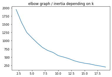
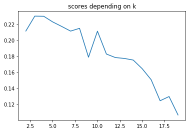
The best nb of k clusters seems to be 8 or 10 even if there isn’t any real elbow on the 1st plot…
So let’s re-train the model with the k number of clusters of 6 :
X = df_wind_transposed

km = KMeans(n_clusters=6).fit(X)
X['label'] = km.labels_
print("Cluster nb / Nb of countries in the cluster", X.label.value_counts())
Cluster nb / Nb of countries in the cluster 3    8
2    8
0    6
5    3
4    2
1    2
Name: label, dtype: int64
Conclusion
At the end, we are able to list the countries in the E.U, countries which share the same profiles when it comes to produces wind energy. To be honest, this was not a difficult task : the data are already cleaned and there is no need to use complicated machine learning here. But knowing the countries with the same characteristics will be usefull for the second step when we will analyze each profile.
You will find below the list of countries in each cluster :
print("Countries grouped by cluster")
for k in range(6):
    print(f'cluster nb : {k}', " ".join(list(X[X.label == k].index)))
Countries grouped by cluster
cluster nb : 0 EE FI LT LV PL SE
cluster nb : 1 ES PT
cluster nb : 2 AT CH CZ HR HU IT SI SK
cluster nb : 3 BE DE DK FR IE LU NL UK
cluster nb : 4 CY NO
cluster nb : 5 BG EL RO
