Computation of Connected Component in Graphs with Spark

Image from Deepmind on Pexels.com.

Implementation of the “CCF: Fast and Scalable Connected Component Computation in MapReduce” paper with Spark. Study of its scalability on several datasets using various clusters’ sizes on Databricks and Google Cloud Platform (GCP)

Table of content

• Abstract
• Description of the CCF algorithm
  • Connected component definition
  • Global methodology
  • Differents steps - counting new pairs
• Spark Implementation
  • Spark Session and context
  • RDD & DataFrame
  • Explanation of each steps
• Scalability Analysis
  • Datasets
  • Computation with Databricks
  • Computation using Google Cloud Dataproc
  • Computation using the LAMSADE cluster
• Conclusion
• Appendix
• References

Abstract

A graph is a mathematical structure used to model pairwise relations between objects. It is made up of vertices (also called nodes or points) which are connected by edges (also called links or lines).
Many practical problems can be represented by graphs: they can be used to model many types of relations and processes in physical, biological, social and information systems. Finding connected components in a graph is a wellknown problem in a wide variety of application areas. For that purpose; in 2014, H. Kardes, S. Agrawal, X. Wang and A. Sun published “CCF: Fast and scalable connected component computation in MapReduce”. Hadoop MapReduce introduced a new paradigm: a programming model for processing big data sets in a parallel and in a distributed way on a cluster, it involves many read/write operations. On the contrary, by running as many operations as possible in-memory - few years later - Spark has proven to be much more faster and has become de-facto a new standard.
In this study, we explain the algorithm and main concepts behind CCF. Then we make a PySpark inplementatoin. And finally we analyze the scalability of our solution applied on datasets of increasing sizes. The computations are realised on a cluster also of an increasing number of nodes in order to see the evolution of the calculation time. We’ve used the Databricks community edition and Google Cloud Dataproc.

Description of the CCF algorithm

Connected component definition

First, let’s give a formal definition in graph theory context:

• V is the set of vertices
• and E is the set of edges
• G = (V,E) be an undirected graph

Properties

• C = (C1,C2, …,Cn) is the set of disjoint connected components in this graph
• (C1 U C2 U … U Cn) = V
• (C1 intersect C2 intersect … intersect Cn) = void.
• For each connected component Ci in C, there exists a path in G between any two vertices vk and vl where (vk, vl) in Ci.
• Additionally, for any distinct connected component (Ci,Cj) in C, there is no path between any pair vk and vl where vk in Ci, vl in Cj.

Thus, problem of finding all connected components in a graph is finding the C satisfying the above conditions.

Global methodology

Here is how CCF works:

• it takes as input a list of all the edges.
• it returns as an output the mapping (i.e a table) from each node to its corresponding componentID (i.e the smallest node id in each connected component it belongs to)

To this end, the following chain of operations take place:

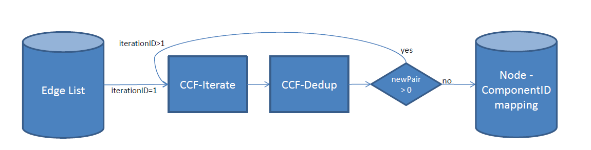
Two jobs run iteratively till we don’t find any new connected peer attached to the existing components:

• CCF-Iterate

This job generates an adjacency lists AL = (a1, a2, …, an) for each node v i.e the list of new nodes belonging to the same connected component. Each time, the node id is eventually updated in case of a new peer node with an id that become the new minimum.
If there is only one node in AL, it means we will generate the pair that we have in previous iteration. However, if there is more than one node in AL, it means that the process is not completed yet: an other iteration is needed to find other peers.

• CCF-Dedup

During the CCF-Iterate job, the same pair might be emitted multiple times. The second job, CCF-Dedup, just deduplicates the output of the CCF-Iterate job in order to improve the algorithm’s efficiency.

Differents steps - counting new pairs

Let’s break the whole process piece by piece using the example illustrated below:

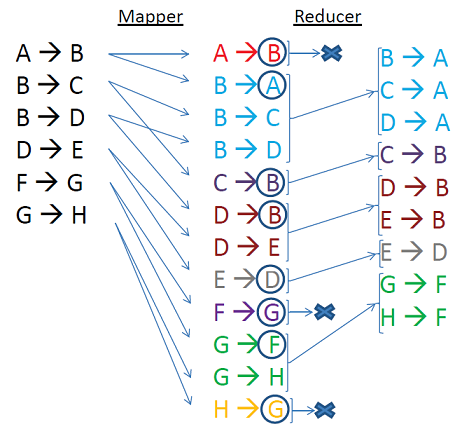
• For each edge, the CCT-Iterate mapper emits both (k, v) and (v, k) pairs so that a should be in the adjacency list of b and vice versa.
• In reduce phase, all the adjacent nodes are grouped together –> pairs are sorted by keys
• All the values are parsed group by group:
  • a first time to find the the minValue
  • a second time to emit a new componentID if needed
• The global NewPair counter is initialized to 0. For each component if a new peer node is found, the counter is incremented. At the end of the job, if the NewPair is still 0: it means that there is not any new edge that can be attached to the existing components: the whole computation task is over. Otherwise an other iteration is needed.

Then we just have to calculate the number of connected components by counting the distinct componentIDs.

Spark Implementation

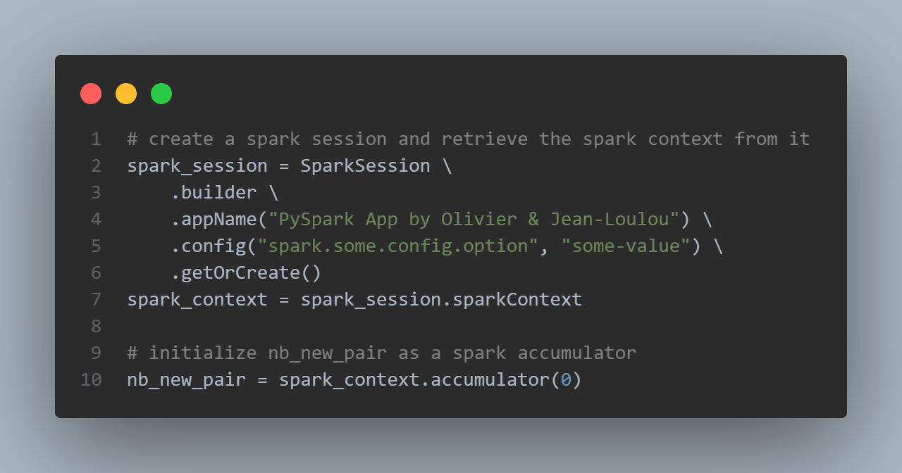
Spark Session and context

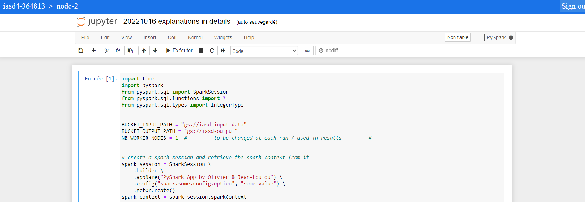
First we create a Spark Session:

Spark applications run as independent sets of processes on a cluster, coordinated by the SparkContext object in your main program (called the driver program).

Spark Driver manage the whole application. It decides what part of job will be done on which Executor and also gets the information from Executors about task statuses.

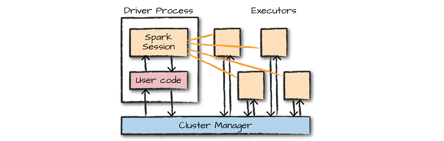
Since earlier versions of Spark or Pyspark, SparkContext (JavaSparkContext for Java) is an entry point to Spark programming with RDD and to connect to Spark Cluster, Since Spark 2.0 SparkSession has been introduced and became an entry point to start programming with DataFrame and Dataset.

An accumulator is used as an excrementing variable to count new pairs:

# initialize nb_new_pair as a spark accumulator
nb_new_pair = sc.accumulator(0)

[...]

def iterate_reduce_df(df):
    [...]
    nb_new_pair += df.withColumn("count", size("v")-1).select(sum("count")).collect()[0][0]
    [...]
...

Accumulators are created at driver program by calling Spark context object. Then accumulators objects are passed along with other serialized tasks code to distributed executors. Task code updates accumulator values. Then Spark sends accumulators back to driver program, merges their values obtained from multuple tasks, and here we can use accumulators for whatever purpose (e.g. reporting). Important moment is that accumulators become accessible to driver code once processing stage is complete.

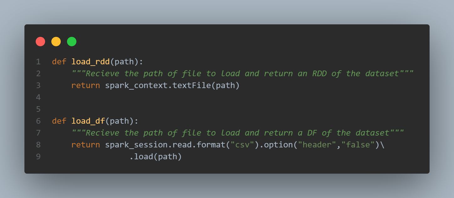
We use the SparkSession to load the dataset into a DataFrame and the SparkContext to use it with RDD.

As you can see the first few lines of headers starting with ‘#’ are not well interpreted, and so is the separator ‘\t’:

rdd_raw = load_rdd(path)
rdd_raw.take(6)

['# bla bla', '# header', '1\t2', '2\t3', '2\t4', '4\t5']

The same issue occurs for with a dataframe:

df_raw = load_df(path)
df_raw.show(6)

+---------+
|      _c0|
+---------+
|# bla bla|
| # header|
|      1	2|
|      2	3|
|      2	4|
|      4	5|
+---------+
only showing top 6 rows

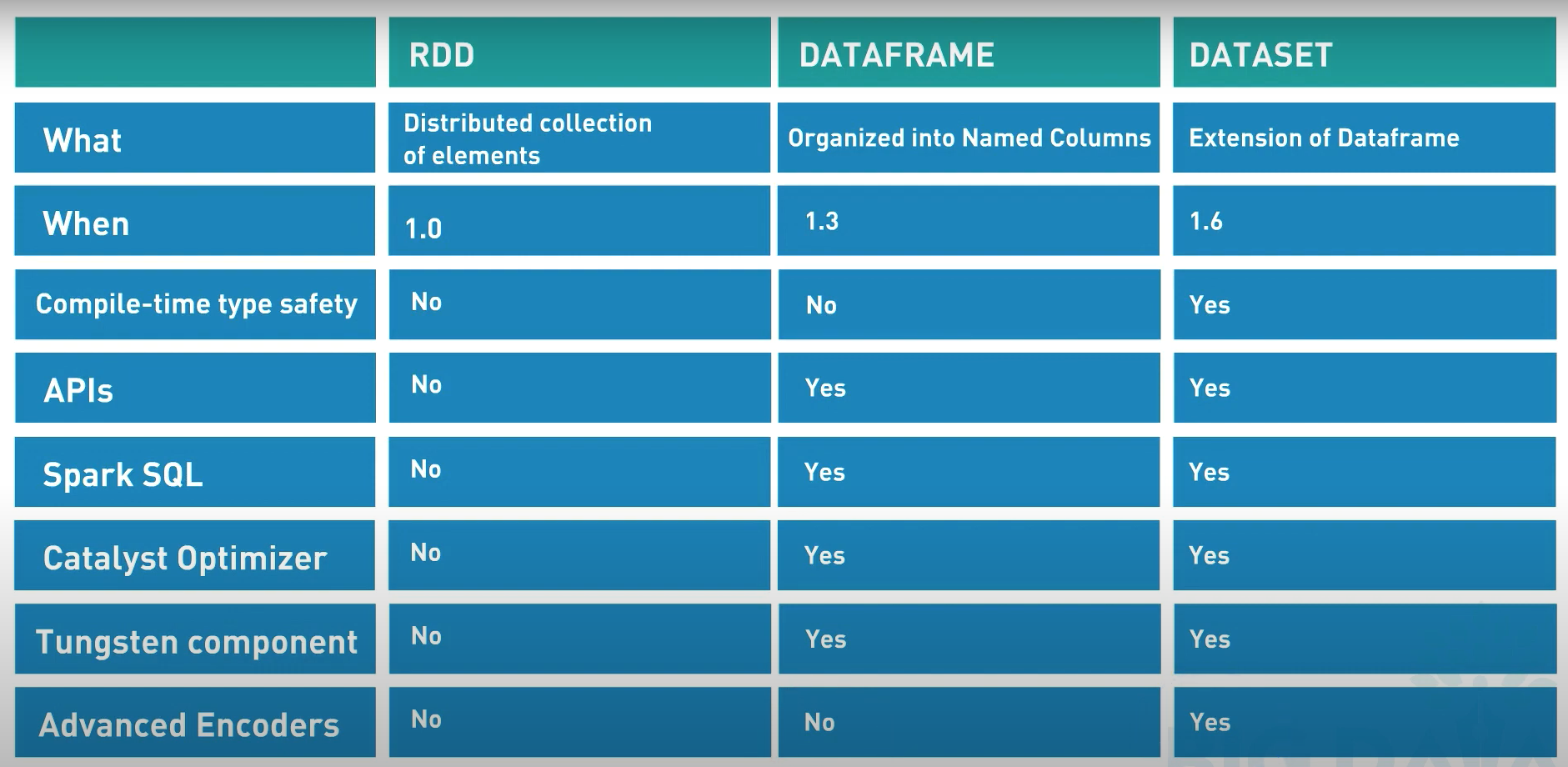
RDD & DataFrame

The RDDs are defined as the distributed collection of the data elements without any schema operating at low level. The Dataframes are defined as the distributed collection organized into named columns with a schema (but without being strongly typed like the Datasets).

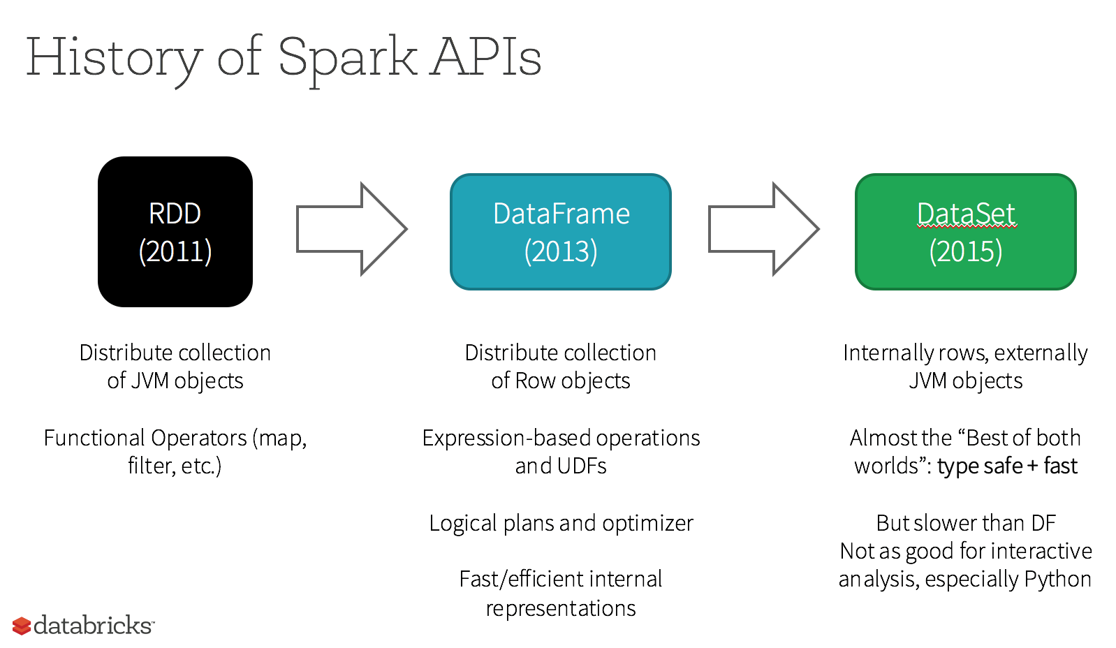
Here is a more exhaustive lists of the differences:

They are considered “resilient” because the whole lineage of data transformations can be rebuild from the DAG if we loose an executor for instance.

Before computation of connected components we prepare the datasets by removing multiline headers and split the two columns separated by a tabulation:

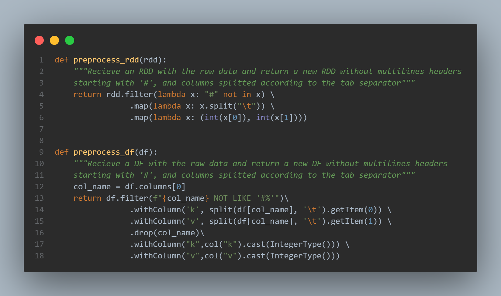
We also cast the informations to integers to get a clean list of (keys, values) in the RDD:

rdd = preprocess_rdd(rdd_raw)
rdd.take(10)

[(1, 2), (2, 3), (2, 4), (4, 5), (6, 7), (7, 8)]

and a ready-to-use table in a Dataframe:

df = preprocess_df(df_raw)
df.show(10)

+---+---+
|  k|  v|
+---+---+
|  1|  2|
|  2|  3|
|  2|  4|
|  4|  5|
|  6|  7|
|  7|  8|
+---+---+

Explanation of each steps

The mapper & reducer jobs illustrated in the picture seen previously (see “Differents steps - counting new pairs”) correspond to the first iteration of the following graph :

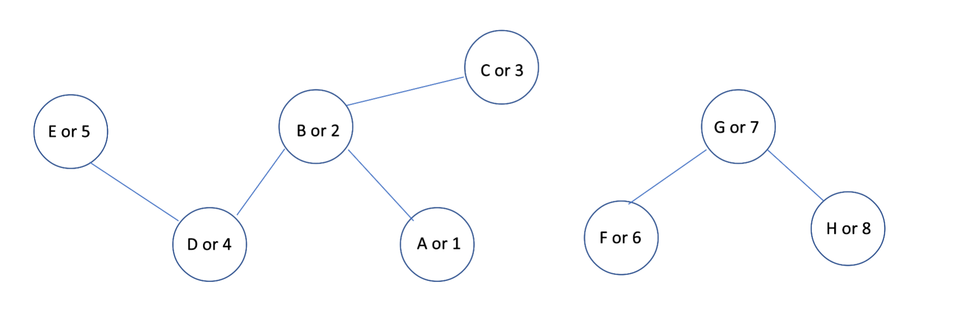
For the sake of clarity, we are going to replace the vertices A by 1, B by 2 and so on… And for each steps, let’s see both the RDD and DataFrame outputs. The computation part starts with the “iterate map” function, its goal is to generate an exhaustive list of edges:

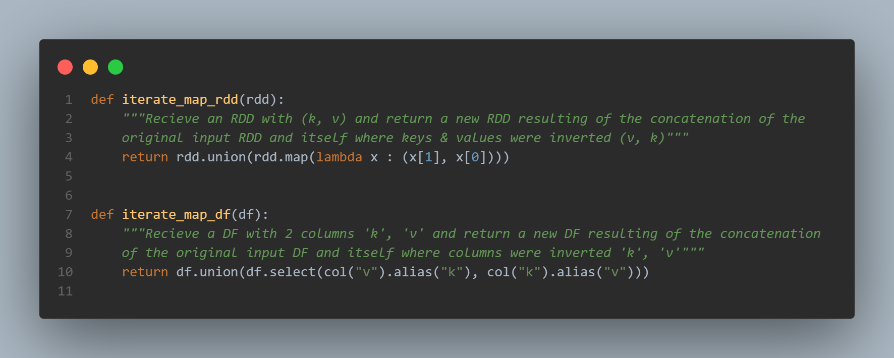
The way to proceed is the same for RDDs or Dataframe: .union is used to concatenate the original RDD or DF with the inverted one. The reversal is achieved by mapping keys / values in a different order for RDDs : rdd.map(lambda x : (x[1], x[0])) et by selecting the columns in a different order for DFs : df.select(col("v").alias("k"), col("k").alias("v")) alias allows us to rename properly columns’ names:

rdd = iterate_map_rdd(rdd)
rdd.take(20)

[(1, 2),
 (2, 3),
 (2, 4),
 (4, 5),
 (6, 7),
 (7, 8),
 (2, 1),
 (3, 2),
 (4, 2),
 (5, 4),
 (7, 6),
 (8, 7)]

The output is quite similar with a Dataframe but with named columns:

df = iterate_map_df(df)
df.show(20)

+---+---+
|  k|  v|
+---+---+
|  1|  2|
|  2|  3|
|  2|  4|
|  4|  5|
|  6|  7|
|  7|  8|
|  2|  1|
|  3|  2|
|  4|  2|
|  5|  4|
|  7|  6|
|  8|  7|
+---+---+

CCF-Iterate job generates adjacency lists AL = (a-1, a-2, …, a-n) for each node v, and if the node id of this node v-id is larger than the min node id a-min in the adjacancy list, it first creates a pair (v-id, a-min) and then a pair for each (a-i, a-min) where a-i 2 AL, and a-i 6 = amin. If there is only one node in AL, it means we will generate the pair that we have in previous iteration.

However, if there is more than one node in AL, it means we might generate a pair that we didn’t have in the previous iteration, and one more iteration is needed.

Nota: if v-id is smaller than a-min, we do not emit any pair.
The pseudo code of CCF-Iterate provided in the original paper is quite similar to the count_nb_new_pair() implementation. We use this function in conjuction of a .groupByKey() and a .flatMap applied on RDDs:

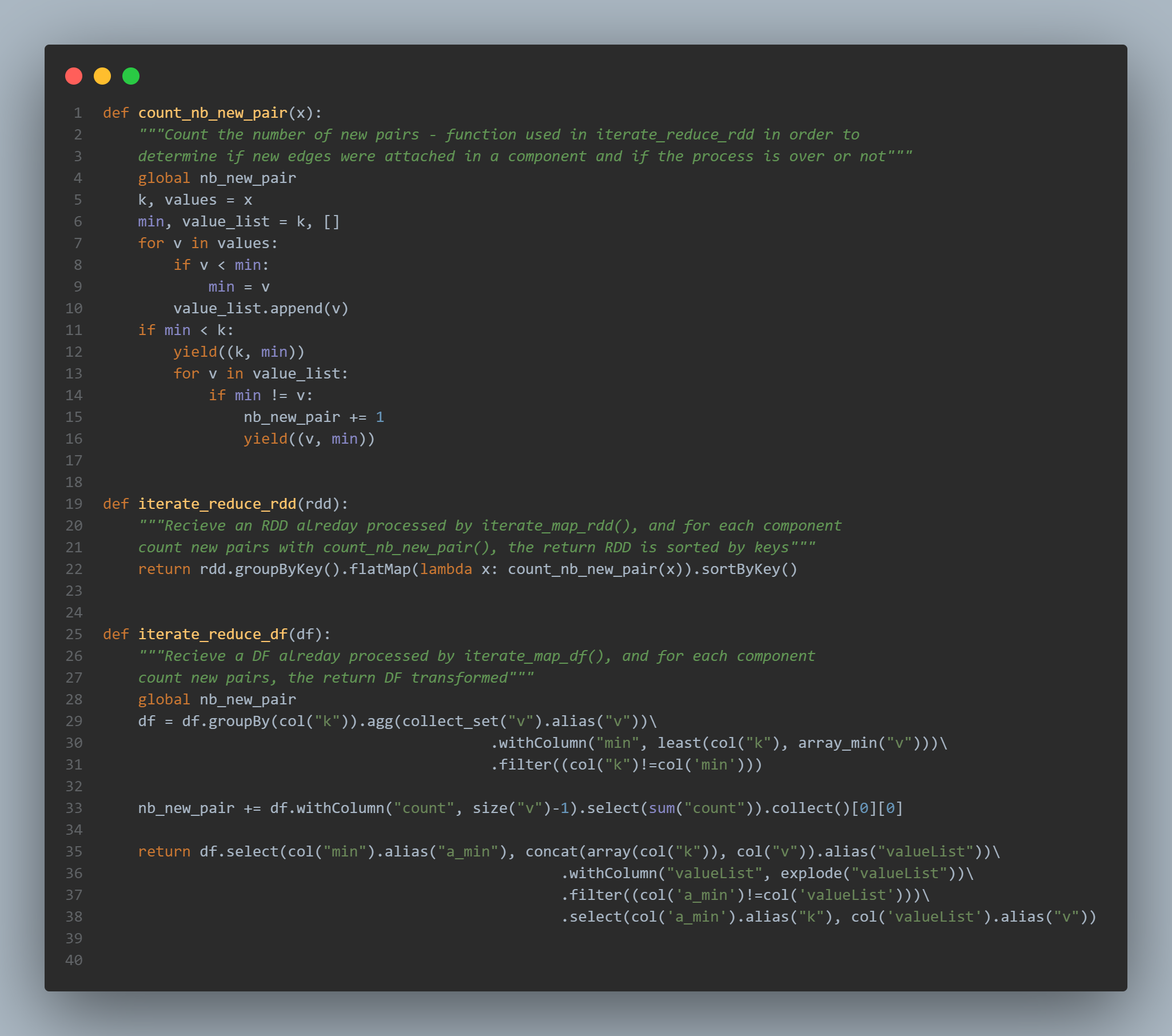
With a dataframe, the main concept remains the same. But the way to count new pairs is a little bit different. We aggregate rows and group them by the column k for key in our case. We determine the min of the values with array_min("v"). Then we sum the count obtained with size("v"):

rdd = iterate_reduce_rdd(rdd)
rdd.take(16)

[(2, 1),
 (3, 1),
 (3, 2),
 (4, 2),
 (4, 1),
 (5, 2),
 (5, 4),
 (7, 6),
 (8, 7),
 (8, 6)]

Similar results with dataframes:

df = iterate_reduce_df(df)
df.show()

+---+---+
|  k|  v|
+---+---+
|  2|  3|
|  4|  5|
|  2|  4|
|  2|  5|
|  6|  7|
|  6|  8|
|  7|  8|
|  1|  2|
|  1|  3|
|  1|  4|
+---+---+

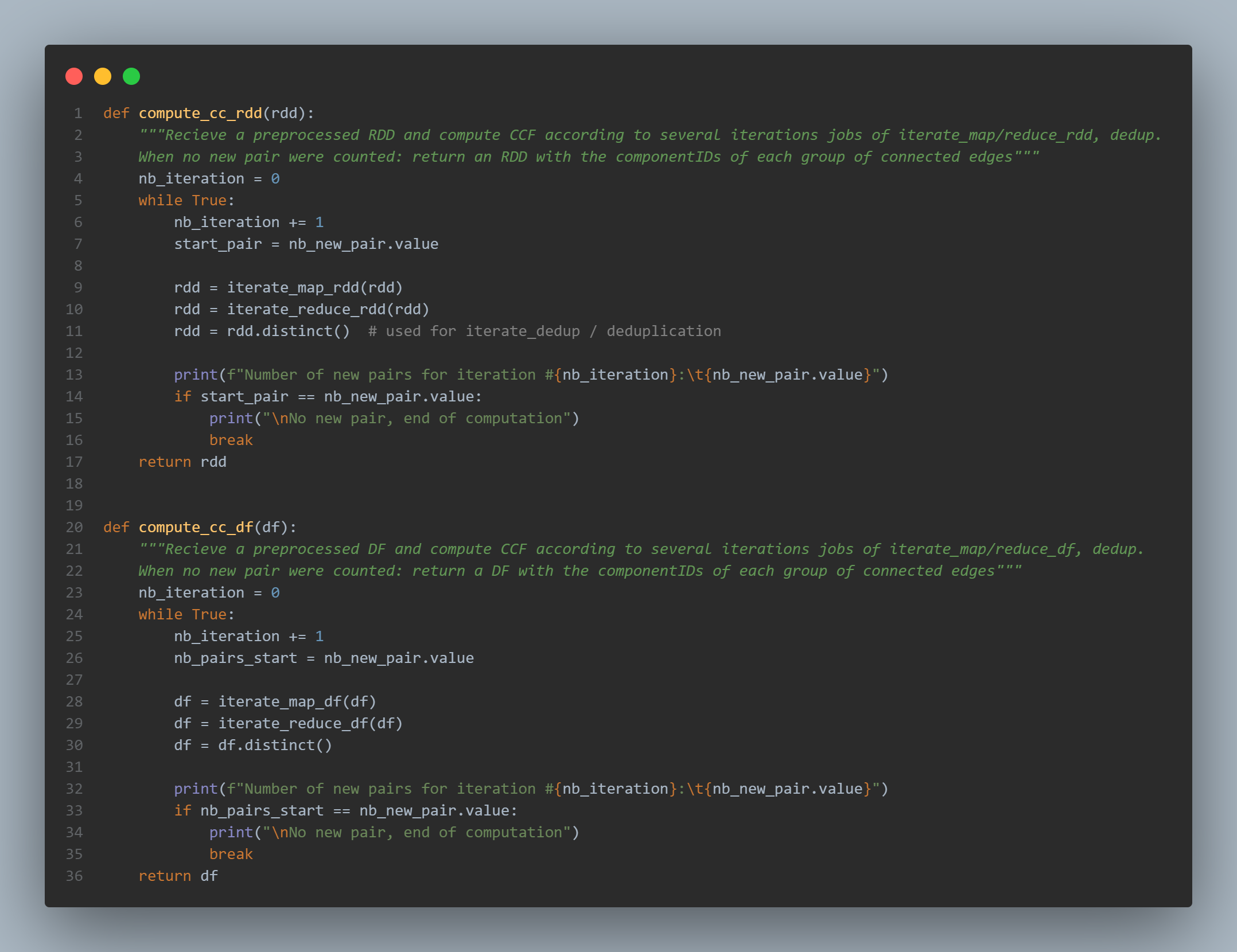
The compute_cc_rdd and compute_cc_df are exactly the same.

• the number of iteration is initialized to zero
• a while loop takes place: if the number of pair at the beginning of the iteration remains unchanged at the end, we break in order to stop the loop. This is done with the condition if start_pair == nb_new_pair.value:. More precisely, the accumulator nb_new_pairis used as an incremental variable. If we want to compute the real number of new pairs, we have to set the values back to zero at the beginning of each iteration and check if the value is not nul at the end.
• as explained in the CCF algorithm paper, the jobs in the loop are:
  • iterate_map
  • iterate_reduce
  • and iterate_dedup (the deduplication is simply achieved using rdd.distinct() or df.distinct())

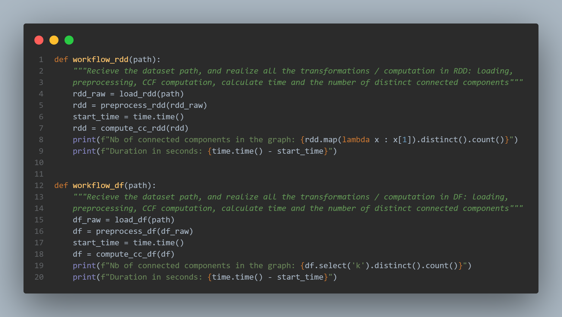
Finally, the workflow_rdd() and workflow_df() functions are just wrappers containing all the previously seen functions:

• the dataset loading with load_rdd(path) and load_df(path)
• its preprocessing with preprocess_rdd(df_raw) and preprocess_df(df_raw)
• then the timer is started: start_time = time.time()
• after that, the computation of the connected components is launched df = compute_cc_df(df) / rdd = compute_cc_rdd(df)
• we print the number of connected components in the graph equal to df.select('k').distinct().count() (same code for RDDs
• and finally, we dispaly the duration in seconds which is equal to the delta: time.time() - start_time

Side note:

Here we don’t include in the timer the reading of the dataset. This time of reading can be decreased with more nodes in the clusters because of the redundancy of the data / distributed storage according to the Hadoop / HDFS replication factor (by default 3). But this is actually not what we’re interested in. On the contrary, the computed number of distinct components should be counted in the duration, because it is our final objective.

Scalability Analysis

We use datasets and Hadoop clusters with Spark both of increasing sizes.

Datasets

Source: Stanford Large Network Dataset Collection web site

Name	Type	Nodes	Edges	Description	Collection date
web-Stanford	Directed	281k	2,3M	Web graph of Stanford.edu	2002
web-NotreDame	Directed	325k	1,5M	Web graph of Notre Dame	1999
web-Google	Directed	875k	5,1M	Web graph from Google	2002
web-BerkStan	Directed	685k	7,6M	Web graph of Berkeley and Stanford	2002

Datasets information

Nodes represent pages and directed edges represent hyperlinks between them for

• Stanford University (stanford.edu)
• University of Notre Dame (domain nd.edu)
• Berkely.edu and Stanford.edu domains
• Web pages released in by Google as a part of Google Programming Contest.

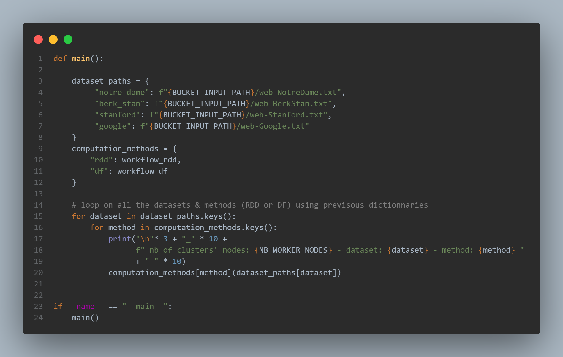
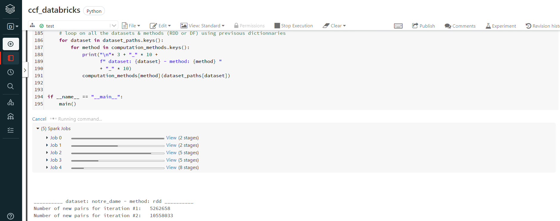
A for loop in the main function parse all the datasets one by one, and for each dataset the CC are computed using RDDs then Dataframes:

Computation with Databricks

• we create a cluster with the following settings available for community edition : 1 Driver: 15.3 GB Memory, 2 Cores, 1 DBU (A Databricks Unit is a normalized unit of processing power on the Databricks Lakehouse Platform used for measurement and pricing purposes. The number of DBUs a workload consumes is driven by processing metrics, which may include the compute resources used and the amount of data processed)

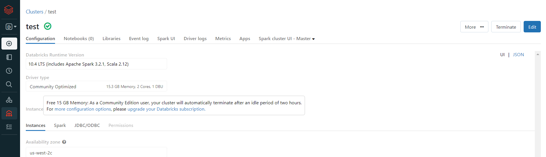
• then we create a table on this cluster and upload our datasets

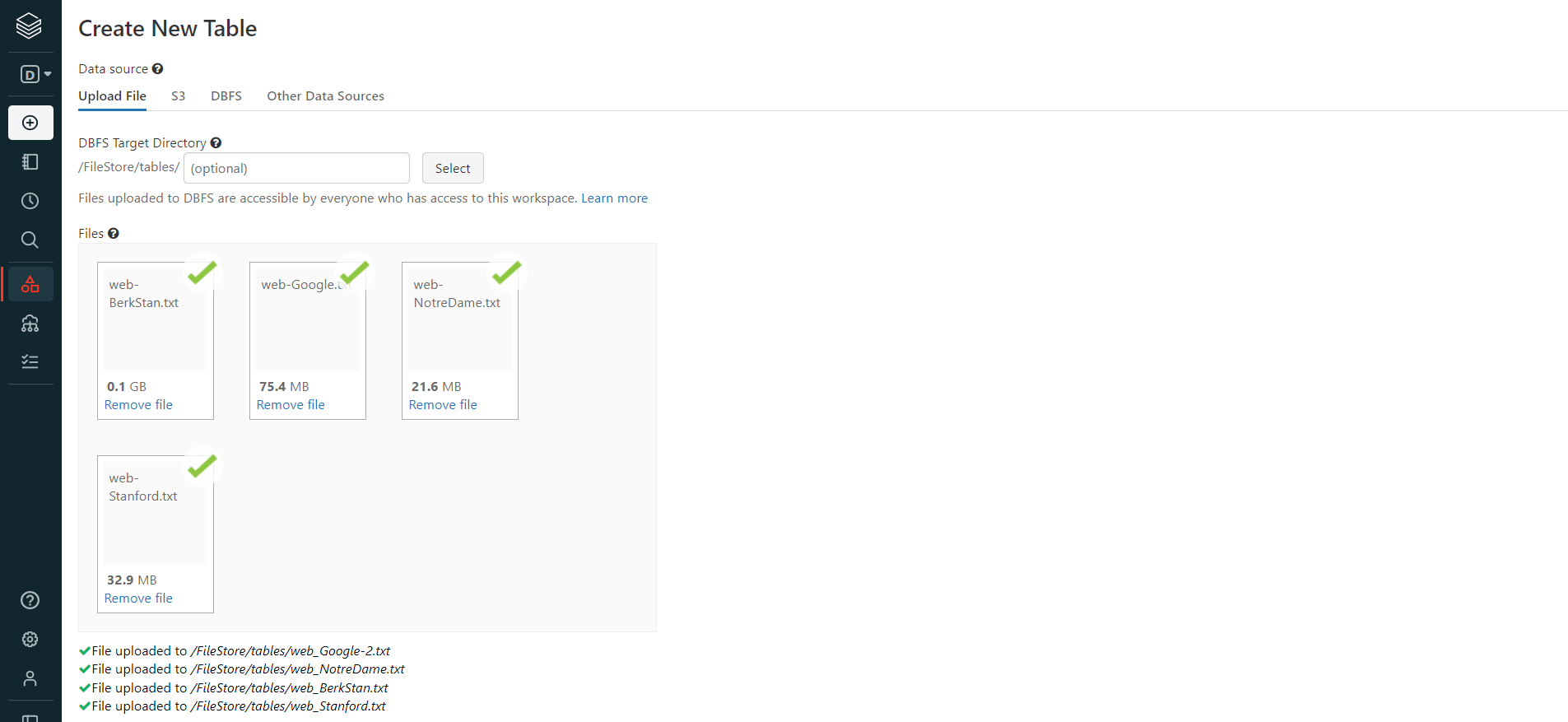
• finally, we run our script in a notebook

The python script is identical to the one used on GCP: only the path of the various datasets were

Computation using Google Cloud Dataproc

Cluster creation

• create buckets with your input data and scripts
• enable Dataproc API
• create a cluster with the following settings:
  • from the web UI with the options below:
    • Enable component gateway
    • Jupyter Notebook
    • the nodes configurations
    • a scheduled deletion of the cluster after an idle time period without submitted jobs
    • Allow API access to all Google Cloud services in the same project.
  • or in command line:

gcloud dataproc clusters create node-2 \
    --enable-component-gateway \
    --region us-central1 \
    --zone us-central1-c \
    --master-machine-type n1-standard-2 \
    --master-boot-disk-size 500 \
    --num-workers 2 \
    --worker-machine-type n1-standard-4  \
    --worker-boot-disk-size 500  \
    --image-version 2.0-debian10  \
    --optional-components JUPYTER  \
    --max-idle 3600s  \
    --scopes 'https://www.googleapis.com/auth/cloud-platform'  \ 
    --project iasd4-364813

3 ways to launch a job

• notebook (for the developpement / analysis part)

• Web UI

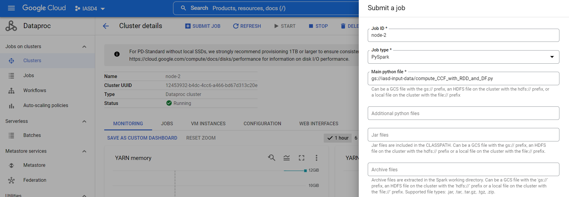
we can add properties to specify the excecutor’s memory & cores number (but it seems that we need to have 1 executor per node otherwise we encounter OOM especially for dataset “BerkStan”):

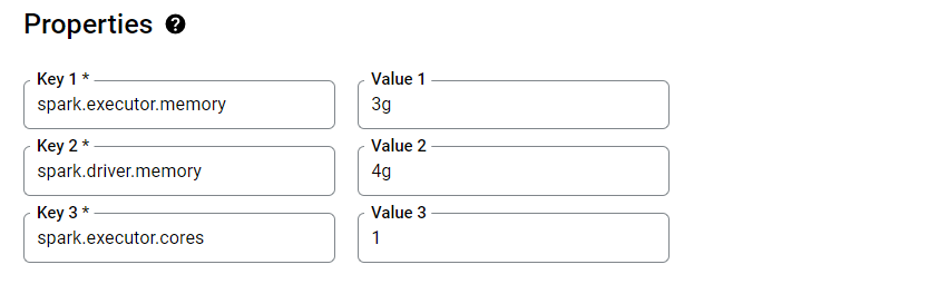
• the GCP equivalent spark submit command where shell variable starting with $ must be initialized and the path_main.pychanged by the URL of the script in the GCS’ bucket: gs://iasd-input-data/compute_CCF_with_RDD_and_DF.py

gcloud dataproc jobs submit pyspark path_main.py \
    --cluster=$CLUSTER_NAME \
    --region=$REGION \
    --properties="spark.submit.deployMode"="cluster",\
    "spark.dynamicAllocation.enabled"="true",\
    "spark.shuffle.service.enabled"="true",\
    "spark.executor.memory"="15g",\
    "spark.driver.memory"="16g",\
    "spark.executor.cores"="5"

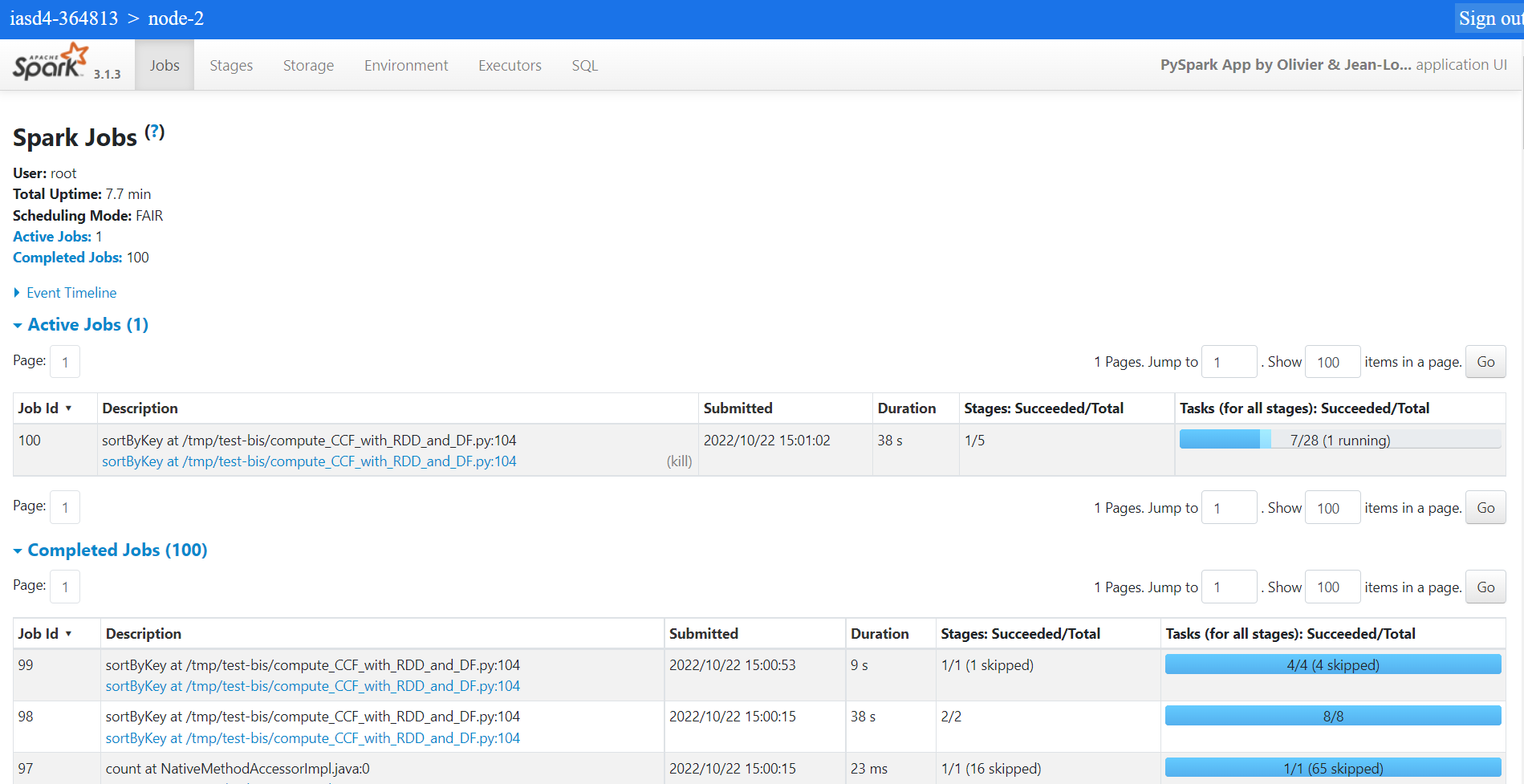
Once a job is submitted, we check its status in Yarn application manager

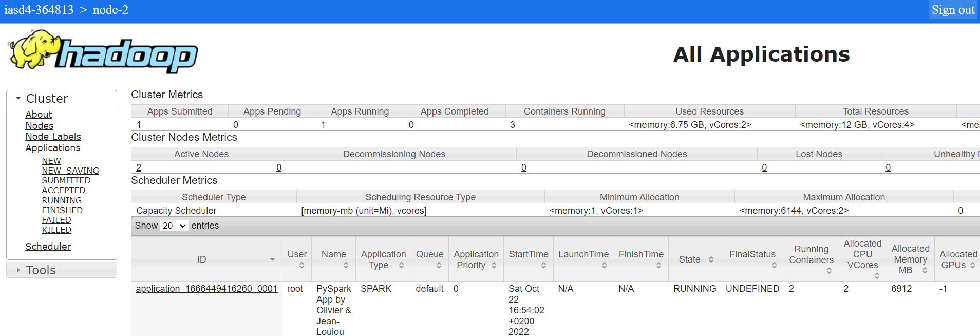
and get into the spark’s details (stages, jobs…)

Computation using the LAMSADE cluster

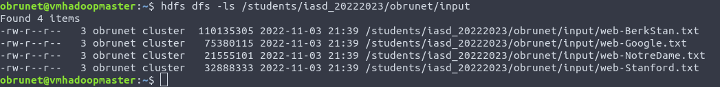
We add our private ssh key and connect to the master node of the LAMSADE’s hadoop cluster. With the linux command line, the archives are directly downloaded using wget, then unzip and putin HDFS:

This cluster comes with Spark version 3.2.0 as showned in the spark-shell:

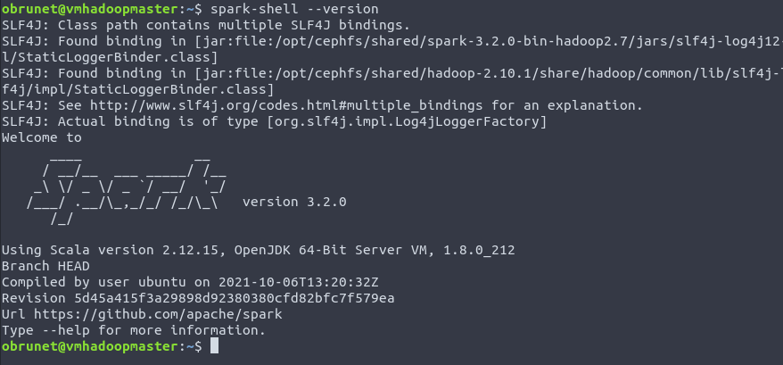
The previous script used with Google Cloud Platform is slightly modified:

• the datasets’ paths are changed with the Hadoop Distributed File System
• the pattern “###” is used before prints in order to easily filter with grep the relevent informations in the spark-submitresults:

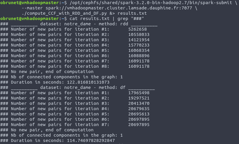
Here is the command used to launch jobs:

/opt/cephfs/shared/spark-3.2.0-bin-hadoop2.7/bin/spark-submit \
	--master spark://vmhadoopmaster.cluster.lamsade.dauphine.fr:7077 \
	./compute_CCF_with_RDD_and_DF.py &> results.txt

spark-submit prints most of it’s output to STDERR. To redirect the entire output to one file, you can use:

spark-submit something.py > results.txt 2>&1
# or
spark-submit something.py &> results.txt

Side note:
We haven’t found the exact number of slaves nodes in the cluster configuration (core-site.xml): the hosts files and some hdfs commands are not accessibles to us with our account / low rights (for security reasons). But it seems that the whole cluster is virtualized on a single big VM with 9 slaves for spark:

obrunet@vmhadoopmaster:/opt/cephfs/shared/spark-3.2.0-bin-hadoop2.7/conf$ cat slaves
vmhadoopslave1
vmhadoopslave2
vmhadoopslave3
vmhadoopslave4
vmhadoopslave5
vmhadoopslave6
vmhadoopslave7
vmhadoopslave8
vmhadoopslave9

Conclusion

Recap of the clusters used:

Name	Master node	Worder node
Databricks	N/C	N/C
GCP 2 nodes	1 x n1-standard-2 (2 vCPU / 7.5GB RAM / 500GB disk)	2 x n1-standard-2 (2 vCPU / 7.5GB RAM / 500GB disk)
Lamsade cluster	at least 1 MN (conf. N.C)	9 slaves (conf. N.C)

Summary of the calculation times in seconds for both resilient distributed datasets and dataframes (rdd / df):

Name	Databricks Com. Ed.	GCP Dataproc 2 nodes	Lamsade cluster 9 slaves
web-Stanford	(*)	12872 / 10565	6375 / 6259
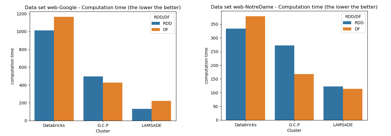
web-NotreDame	333 / 379	272 / 168	122 / 114
web-Google	1012 / 1165	497 / 425	132 / 222
web-BerkStan	N/A (**)	N/A (**)	N/A (**)

(*) lasts too long: result not recorded
(**) the web-BerkStan is finally a single connected component with too many edges with regard to the number of vertices (unfortunately this couldn’t be guessed before the end of the computation!): it causes out of memory errors occuring in executors for the GCP Dataproc and no space left on the device problems for the driver of the LAMSADE cluster.

Comparison of results

Comments about this experimental analysis

• Even if RDDs operate at a lower level - our first intuition was that computation with RDDs will take less time - this is not always true. In the table above there are few cases where using DFs lead to faster results.
• The Databricks community edition use a single VM, while the Google Cloud involve 2 worker nodes and the LAMSADE cluster 9 slaves: we can clearly see that with more nodes, the computation takes less time (whether with RDDs or DFs). The parallelism of operations such as map, filter or reduce… significantly improves performances.
• One can notice that if you run the same script twice in the same conditions i.e on the same dataset with the same cluster, you can get slightly different results: this can be a consequence of
  • shared ressources for the LAMSADE cluster
  • we could assume the way partitions are dispatched can have an impact: if the same connected component is computed on several nodes because each slave is dealing with different vertices (of the same component), it will take more time than after a shuffle. So graph with very few connected components might be affected (see the web-BerkStan dataset)

Strenghts and weaknesses of the algorithm

• It makes use of a loop, which is not in accordance with the distributed processing paradigm but to our knowledge we can’t proceed without any loop.
• It is not suited for “highly” connected graphs with a high ratio of vertices compared to edges.
• As stated previously, the computation time is influenced by the way the data / partitions are splitted among nodes of the cluster. The same run can lead to a different number of iterations, the lack of reproductibility could also be an issue.
• Nevertheless, finding connected components in graph remains a complex task, the CCF algorithm has proven to be a robust solution, further more a solution that can be parallelized.

Alternative solutions

One also might consider using the spark’s graphx librairy (not maintained anymore & only in Scala) or graph databases such as Neo4J or specific librairies like NetworkX.

Appendix

• PySpark Script run on GCP Dataproc
• Notebook with the explanations in depth
• Databricks notebook - online & local archive
• PySpark Script run on the LAMSADE cluster

References

Paper

• “CCF: Fast and scalable connected component computation in MapReduce”
• Local archive

Datasets

• Stanford Large Network Dataset Collection web site
  • Web graph of Berkeley and Stanford
  • Web graph from Google
  • Web graph of Notre Dame
  • Web graph of Stanford.edu

Documentation

• Latest version of Spark
• Databricks community edition
• Google Cloud Dataproc