Solar energy generation 1/3 - clustering countries & regions

Description of the data set

This dataset contains hourly estimates of an area’s energy potential for 1986-2015 as a percentage of a power plant’s maximum output.

The overall scope of EMHIRES is to allow users to assess the impact of meteorological and climate variability on the generation of solar power in Europe and not to mime the actual evolution of solar power production in the latest decades. For this reason, the hourly solar power generation time series are released for meteorological conditions of the years 1986-2015 (30 years) without considering any changes in the solar installed capacity. Thus, the installed capacity considered is fixed as the one installed at the end of 2015. For this reason, data from EMHIRES should not be compared with actual power generation data other than referring to the reference year 2015.

Content

• The data is available at both the national level and the NUTS 2 level. The NUTS 2 system divides the EU into 276 statistical units.
• Please see the manual for the technical details of how these estimates were generated.
• This product is intended for policy analysis over a wide area and is not the best for estimating the output from a single system. Please don’t use it commercially.

Acknowledgements

This dataset was kindly made available by the European Commission’s STETIS program. You can find the original dataset here.

Goal of this 1st step

This is the first part of three. Here we’re going to study solar generation on a country level in order to make cluster of country which present the same profile so that each group can be investigate in more details later.

# import of needed libraries

import numpy as np
import pandas as pd
from scipy import stats
import seaborn as sns
import matplotlib.pyplot as plt

pd.options.display.max_columns = 300

import warnings
warnings.filterwarnings("ignore")

First let’s start with the data set for each country :

# let's see what our data set look like

df_solar_co = pd.read_csv("solar_generation_by_country.csv")
df_solar_co.head(2)

	AT	BE	BG	CH	CY	CZ	DE	DK	EE	ES	FI	FR	EL	HR	HU	IE	IT	LT	LU	LV	NL	NO	PL	PT	RO	SI	SK	SE	UK
0	0.0	0.0	0.0	0.0	0	0.0	0.0	0.0	0.0	0.0	0.0	0.0	0.0	0.0	0.0	0.0	0.0	0.0	0.0	0.0	0.0	0.0	0.0	0.0	0.0	0.0	0.0	0.0	0.0
1	0.0	0.0	0.0	0.0	0	0.0	0.0	0.0	0.0	0.0	0.0	0.0	0.0	0.0	0.0	0.0	0.0	0.0	0.0	0.0	0.0	0.0	0.0	0.0	0.0	0.0	0.0	0.0	0.0

Each column represent a country, we can list them easily :

df_solar_co.columns

Index(['AT', 'BE', 'BG', 'CH', 'CY', 'CZ', 'DE', 'DK', 'EE', 'ES', 'FI', 'FR',
       'EL', 'HR', 'HU', 'IE', 'IT', 'LT', 'LU', 'LV', 'NL', 'NO', 'PL', 'PT',
       'RO', 'SI', 'SK', 'SE', 'UK'],
      dtype='object')

If needed, here is a dictionnary in python that can help us to make the conversion between the 2 letters and the real name of each country :

country_dict = {
'AT': 'Austria',
'BE': 'Belgium',
'BG': 'Bulgaria',
'CH': 'Switzerland',
'CY': 'Cyprus',
'CZ': 'Czech Republic',
'DE': 'Germany',
'DK': 'Denmark',
'EE': 'Estonia',
'ES': 'Spain',
'FI': 'Finland',
'FR': 'France',
'EL': 'Greece',
'UK': 'United Kingdom',
'HU': 'Hungary',
'HR': 'Croatia',
'IE': 'Ireland',
'IT': 'Italy',
'LT': 'Lithuania',
'LU': 'Luxembourg',
'LV': 'Latvia',
'NO': 'Norway',
'NL': 'Netherlands',
'PL': 'Poland',
'PT': 'Portugal',
'RO': 'Romania',
'SE': 'Sweden',
'SI': 'Slovenia',
'SK': 'Slovakia'
    }

How many columns and lines of records do we have :

df_solar_co.shape

(262968, 29)

Then, let’s take a look at the data set at the NUTS 2 level system :

df_solar_nu = pd.read_csv("solar_generation_by_station.csv")
df_solar_nu = df_solar_nu.drop(columns=['time_step'])
df_solar_nu.tail(2)

	AT11	AT21	AT12	AT31	AT32	AT22	AT33	AT34	AT13	BE21	BE31	BE32	BE33	BE22	BE34	BE35	BE23	BE10	BE24	BE25	BG32	BG33	BG31	BG34	BG41	BG42	CZ06	CZ03	CZ08	CZ01	CZ05	CZ04	CZ02	CZ07	DEA5	DE30	DE40	DE91	DE50	DED1	DE71	DEE1	DEA4	DED2	DEA1	DE13	DE72	DEE2	DE60	DE92	DE12	DE73	DEB1	DEA2	DED3	DE93	DEE3	DE80	DE25	DEA3	DE22	DE21	DE24	DE23	DEB3	DEF0	DE27	DE11	DEG0	DEB2	DE14	DE26	DE94	ES61	ES24	ES12	ES13	ES41	ES42	ES51	ES30	ES52	ES43	ES11	ES53	ES23	ES22	ES21	ES62	FI20	FI1C	FI1D	FI1B	FI19	FR42	FR61	FR72	FR25	FR26	FR52	FR24	FR21	FR83	FR43	FR23	FR10	FR81	FR63	FR41	FR62	FR30	FR51	FR22	FR53	FR82	FR71	EL51	EL30	EL63	EL53	EL62	EL54	EL52	EL43	EL42	EL65	EL64	EL61	EL41	HU33	HU23	HU32	HU31	HU21	HU10	HU22	CH02	CH03	CH05	CH01	CH07	CH06	CH04	IE01	IE02	ITF1	ITF5	ITF6	ITF3	ITH5	ITH4	ITI4	ITC3	ITC4	ITI3	ITF2	ITC1	ITF4	ITG2	ITG1	ITI1	ITH2	ITI2	ITC2	ITH3	NL13	NL23	NL12	NL22	NL11	NL42	NL41	NL32	NL21	NL31	NL34	NL33	NO04	NO02	NO01	NO03	NO05	PL51	PL61	PL31	PL43	PL11	PL21	PL12	PL52	PL32	PL34	PL63	PL22	PL33	PL62	PL41	PL42	PT18	PT15	PT16	PT17	PT11	RO32	RO12	RO21	RO11	RO31	RO22	RO41	RO42	SE32	SE31	SE12	SE33	SE21	SE11	SE22	SE23	SK01	SK03	SK04	SK02	UKH2	UKJ1	UKD6	UKK3	UKD1	UKF1	UKK4	UKK2	UKH1	UKE1	UKL2	UKM2	UKH3	UKK1	UKD3	UKJ3	UKG1	UKM6	UKI3UKI4	UKJ4	UKD4	UKF2	UKF3	UKD7	UKM5	UKE2	UKN0	UKC2	UKI5UKI6	UKG2	UKM3	UKE3	UKJ2	UKC1	UKG3	UKL1	UKE4
262966	0.0	0.0	0.0	0.0	0.0	0.0	0.0	0.0	0.0	0.0	0.0	0.0	0.0	0.0	0.0	0.0	0.0	0.0	0.0	0.0	0.0	0.0	0.0	0.0	0.0	0.0	0.0	0.0	0.0	0.0	0.0	0.0	0.0	0.0	0.0	0.0	0.0	0.0	0.0	0.0	0.0	0.0	0.0	0.0	0.0	0.0	0.0	0.0	0.0	0.0	0.0	0.0	0.0	0.0	0.0	0.0	0.0	0.0	0.0	0.0	0.0	0.0	0.0	0.0	0.0	0.0	0.0	0.0	0.0	0.0	0.0	0.0	0.0	0.0	0.0	0.0	0.0	0.0	0.0	0.0	0.0	0.0	0.0	0.0	0.0	0.0	0.0	0.0	0.0	0.0	0.0	0.0	0.0	0.0	0.0	0.0	0.0	0.0	0.0	0.0	0.0	0.0	0.0	0.0	0.0	0.0	0.0	0.0	0.0	0.0	0.0	0.0	0.0	0.0	0.0	0.0	0.0	0.0	0.0	0.0	0.0	0.0	0.0	0.0	0.0	0.0	0.0	0.0	0.0	0.0	0.0	0.0	0.0	0.0	0.0	0.0	0.0	0.0	0.0	0.0	0.0	0.0	0.0	0.0	0.0	0.0	0.0	0.0	0.0	0.0	0.0	0.0	0.0	0.0	0.0	0.0	0.0	0.0	0.0	0.0	0.0	0.0	0.0	0.0	0.0	0.0	0.0	0.0	0.0	0.0	0.0	0.0	0.0	0.0	0.0	0.0	0.0	0.0	0.0	0.0	0.0	0.0	0.0	0.0	0.0	0.0	0.0	0.0	0.0	0.0	0.0	0.0	0.0	0.0	0.0	0.0	0.0	0.0	0.0	0.0	0.0	0.0	0.0	0.0	0.0	0.0	0.0	0.0	0.0	0.0	0.0	0.0	0.0	0.0	0	0.0	0.0	0.0	0.0	0.0	0.0	0.0	0.0	0.0	0.0	0.0	0.0	0.0	0.0	0.0	0.0	0.0	0.0	0.0	0.0	0.0	0.0	0.0	0.0	0.0	0.0	0.0	0.0	0.0	0.0	0.0	0.0	0.0	0.0	0.0	0.0	0.0	0.0	0.0	0.0	0.0	0.0	0.0	0.0	0.0
262967	0.0	0.0	0.0	0.0	0.0	0.0	0.0	0.0	0.0	0.0	0.0	0.0	0.0	0.0	0.0	0.0	0.0	0.0	0.0	0.0	0.0	0.0	0.0	0.0	0.0	0.0	0.0	0.0	0.0	0.0	0.0	0.0	0.0	0.0	0.0	0.0	0.0	0.0	0.0	0.0	0.0	0.0	0.0	0.0	0.0	0.0	0.0	0.0	0.0	0.0	0.0	0.0	0.0	0.0	0.0	0.0	0.0	0.0	0.0	0.0	0.0	0.0	0.0	0.0	0.0	0.0	0.0	0.0	0.0	0.0	0.0	0.0	0.0	0.0	0.0	0.0	0.0	0.0	0.0	0.0	0.0	0.0	0.0	0.0	0.0	0.0	0.0	0.0	0.0	0.0	0.0	0.0	0.0	0.0	0.0	0.0	0.0	0.0	0.0	0.0	0.0	0.0	0.0	0.0	0.0	0.0	0.0	0.0	0.0	0.0	0.0	0.0	0.0	0.0	0.0	0.0	0.0	0.0	0.0	0.0	0.0	0.0	0.0	0.0	0.0	0.0	0.0	0.0	0.0	0.0	0.0	0.0	0.0	0.0	0.0	0.0	0.0	0.0	0.0	0.0	0.0	0.0	0.0	0.0	0.0	0.0	0.0	0.0	0.0	0.0	0.0	0.0	0.0	0.0	0.0	0.0	0.0	0.0	0.0	0.0	0.0	0.0	0.0	0.0	0.0	0.0	0.0	0.0	0.0	0.0	0.0	0.0	0.0	0.0	0.0	0.0	0.0	0.0	0.0	0.0	0.0	0.0	0.0	0.0	0.0	0.0	0.0	0.0	0.0	0.0	0.0	0.0	0.0	0.0	0.0	0.0	0.0	0.0	0.0	0.0	0.0	0.0	0.0	0.0	0.0	0.0	0.0	0.0	0.0	0.0	0.0	0.0	0.0	0.0	0	0.0	0.0	0.0	0.0	0.0	0.0	0.0	0.0	0.0	0.0	0.0	0.0	0.0	0.0	0.0	0.0	0.0	0.0	0.0	0.0	0.0	0.0	0.0	0.0	0.0	0.0	0.0	0.0	0.0	0.0	0.0	0.0	0.0	0.0	0.0	0.0	0.0	0.0	0.0	0.0	0.0	0.0	0.0	0.0	0.0

df_solar_nu.shape

(262968, 260)

---

Groups of countries or regions with similar profiles

Clustering with the KMean model

The objective of clustering is to identify distinct groups in a dataset such that the observations within a group are similar to each other but different from observations in other groups. In k-means clustering, we specify the number of desired clusters k, and the algorithm will assign each observation to exactly one of these k clusters. The algorithm optimizes the groups by minimizing the within-cluster variation (also known as inertia) such that the sum of the within-cluster variations across all k clusters is as small as possible.

Different runs of k-means will result in slightly different cluster assignments because k-means randomly assigns each observation to one of the k clusters to kick off the clustering process. k-means does this random initialization to speed up the clustering process. After this random initialization, k-means reassigns the observations to different clusters as it attempts to minimize the Euclidean distance between each observation and its cluster’s center point, or centroid. This random initialization is a source of randomness, resulting in slightly different clustering assignments, from one k-means run to another.

Typically, the k-means algorithm does several runs and chooses the run that has the best separation, defined as the lowest total sum of within-cluster variations across all k clusters.

Reference : Hands-On Unsupervised Learning Using Python

Evaluating the cluster quality

The goal here isn’t just to make clusters, but to make good, meaningful clusters. Quality clustering is when the datapoints within a cluster are close together, and afar from other clusters. The two methods to measure the cluster quality are described below:

• Inertia: Intuitively, inertia tells how far away the points within a cluster are. Therefore, a small of inertia is aimed for. The range of inertia’s value starts from zero and goes up.
• Silhouette score: Silhouette score tells how far away the datapoints in one cluster are, from the datapoints in another cluster. The range of silhouette score is from -1 to 1. Score should be closer to 1 than -1.

Reference : Towards Data Science

Optimal K: the elbow method

How many clusters would you choose ?

A common, empirical method, is the elbow method. You plot the mean distance of every point toward its cluster center, as a function of the number of clusters. Sometimes the plot has an arm shape, and the elbow would be the optimal K.

from sklearn.cluster import KMeans
from sklearn.metrics import silhouette_score

On the NUTS 2 level

Let’s keep the records of one year and tranpose the dataset, because we need to have one line per region.

df_solar_transposed = df_solar_nu[-24*365:].T
df_solar_transposed.tail(2)

	254208	254209	254210	254211	254212	254213	254214	254215	254216	254217	254218	254219	254220	254221	254222	254223	254224	254225	254226	254227	254228	254229	254230	254231	254232	254233	254234	254235	254236	254237	254238	254239	254240	254241	254242	254243	254244	254245	254246	254247	254248	254249	254250	254251	254252	254253	254254	254255	254256	254257	254258	254259	254260	254261	254262	254263	254264	254265	254266	254267	254268	254269	254270	254271	254272	254273	254274	254275	254276	254277	254278	254279	254280	254281	254282	254283	254284	254285	254286	254287	254288	254289	254290	254291	254292	254293	254294	254295	254296	254297	254298	254299	254300	254301	254302	254303	254304	254305	254306	254307	254308	254309	254310	254311	254312	254313	254314	254315	254316	254317	254318	254319	254320	254321	254322	254323	254324	254325	254326	254327	254328	254329	254330	254331	254332	254333	254334	254335	254336	254337	254338	254339	254340	254341	254342	254343	254344	254345	254346	254347	254348	254349	254350	254351	254352	254353	254354	254355	254356	254357	...	262818	262819	262820	262821	262822	262823	262824	262825	262826	262827	262828	262829	262830	262831	262832	262833	262834	262835	262836	262837	262838	262839	262840	262841	262842	262843	262844	262845	262846	262847	262848	262849	262850	262851	262852	262853	262854	262855	262856	262857	262858	262859	262860	262861	262862	262863	262864	262865	262866	262867	262868	262869	262870	262871	262872	262873	262874	262875	262876	262877	262878	262879	262880	262881	262882	262883	262884	262885	262886	262887	262888	262889	262890	262891	262892	262893	262894	262895	262896	262897	262898	262899	262900	262901	262902	262903	262904	262905	262906	262907	262908	262909	262910	262911	262912	262913	262914	262915	262916	262917	262918	262919	262920	262921	262922	262923	262924	262925	262926	262927	262928	262929	262930	262931	262932	262933	262934	262935	262936	262937	262938	262939	262940	262941	262942	262943	262944	262945	262946	262947	262948	262949	262950	262951	262952	262953	262954	262955	262956	262957	262958	262959	262960	262961	262962	262963	262964	262965	262966	262967
UKL1	0.0	0.0	0.0	0.0	0.0	0.0	0.0	0.0	0.0	0.00454	0.03268	0.03582	0.03150	0.03397	0.01626	0.00882	0.00228	0.0	0.0	0.0	0.0	0.0	0.0	0.0	0.0	0.0	0.0	0.0	0.0	0.0	0.0	0.0	0.0	0.06154	0.21109	0.31614	0.38716	0.43612	0.28436	0.12670	0.00333	0.0	0.0	0.0	0.0	0.0	0.0	0.0	0.0	0.0	0.0	0.0	0.0	0.0	0.0	0.0	0.0	0.02394	0.03295	0.03424	0.09291	0.14847	0.14145	0.08795	0.0051	0.0	0.0	0.0	0.0	0.0	0.0	0.0	0.0	0.0	0.0	0.0	0.0	0.0	0.0	0.0	0.0	0.03058	0.14815	0.23625	0.25697	0.19358	0.09569	0.03562	0.00691	0.0	0.0	0.0	0.0	0.0	0.0	0.0	0.0	0.0	0.0	0.0	0.0	0.0	0.0	0.0	0.0	0.01195	0.03161	0.04202	0.05229	0.03885	0.02274	0.02475	0.00777	0.0	0.0	0.0	0.0	0.0	0.0	0.0	0.0	0.0	0.0	0.0	0.0	0.0	0.0	0.0	0.0	0.04288	0.11208	0.23709	0.30366	0.33393	0.25748	0.11807	0.00818	0.0	0.0	0.0	0.0	0.0	0.0	0.0	0.0	0.0	0.0	0.0	0.0	0.0	...	0.0	0.0	0.0	0.0	0.0	0.0	0.0	0.0	0.0	0.0	0.0	0.0	0.0	0.0	0.0	0.01058	0.01703	0.05131	0.03971	0.05035	0.03112	0.00590	0.0	0.0	0.0	0.0	0.0	0.0	0.0	0.0	0.0	0.0	0.0	0.0	0.0	0.0	0.0	0.0	0.0	0.04350	0.13731	0.12993	0.08754	0.10142	0.03618	0.01122	0.0	0.0	0.0	0.0	0.0	0.0	0.0	0.0	0.0	0.0	0.0	0.0	0.0	0.0	0.0	0.0	0.0	0.00540	0.01848	0.02360	0.02316	0.05459	0.09607	0.02429	0.0	0.0	0.0	0.0	0.0	0.0	0.0	0.0	0.0	0.0	0.0	0.0	0.0	0.0	0.0	0.0	0.0	0.06691	0.18368	0.25561	0.27386	0.15795	0.13123	0.05063	0.0	0.0	0.0	0.0	0.0	0.0	0.0	0.0	0.0	0.0	0.0	0.0	0.0	0.0	0.0	0.0	0.0	0.00780	0.01089	0.02214	0.03015	0.03136	0.03555	0.02274	0.00038	0.0	0.0	0.0	0.0	0.0	0.0	0.0	0.0	0.0	0.0	0.0	0.0	0.0	0.0	0.0	0.0	0.02876	0.06367	0.05851	0.05175	0.02705	0.05831	0.04033	0.00142	0.0	0.0	0.0	0.0	0.0	0.0	0.0
UKE4	0.0	0.0	0.0	0.0	0.0	0.0	0.0	0.0	0.0	0.00422	0.05240	0.05711	0.06402	0.07822	0.07162	0.00393	0.00000	0.0	0.0	0.0	0.0	0.0	0.0	0.0	0.0	0.0	0.0	0.0	0.0	0.0	0.0	0.0	0.0	0.06132	0.22173	0.31866	0.34098	0.26557	0.23731	0.04649	0.00000	0.0	0.0	0.0	0.0	0.0	0.0	0.0	0.0	0.0	0.0	0.0	0.0	0.0	0.0	0.0	0.0	0.00084	0.01680	0.00704	0.03624	0.09647	0.16272	0.02156	0.0000	0.0	0.0	0.0	0.0	0.0	0.0	0.0	0.0	0.0	0.0	0.0	0.0	0.0	0.0	0.0	0.0	0.09211	0.30877	0.45304	0.50767	0.42091	0.31502	0.12314	0.00000	0.0	0.0	0.0	0.0	0.0	0.0	0.0	0.0	0.0	0.0	0.0	0.0	0.0	0.0	0.0	0.0	0.09572	0.24905	0.29321	0.33915	0.20611	0.12507	0.00189	0.00000	0.0	0.0	0.0	0.0	0.0	0.0	0.0	0.0	0.0	0.0	0.0	0.0	0.0	0.0	0.0	0.0	0.04483	0.03067	0.07332	0.09302	0.23959	0.22082	0.08960	0.00000	0.0	0.0	0.0	0.0	0.0	0.0	0.0	0.0	0.0	0.0	0.0	0.0	0.0	...	0.0	0.0	0.0	0.0	0.0	0.0	0.0	0.0	0.0	0.0	0.0	0.0	0.0	0.0	0.0	0.00581	0.00787	0.01153	0.08664	0.06156	0.03130	0.02076	0.0	0.0	0.0	0.0	0.0	0.0	0.0	0.0	0.0	0.0	0.0	0.0	0.0	0.0	0.0	0.0	0.0	0.04454	0.31123	0.41020	0.45262	0.41357	0.30795	0.01848	0.0	0.0	0.0	0.0	0.0	0.0	0.0	0.0	0.0	0.0	0.0	0.0	0.0	0.0	0.0	0.0	0.0	0.00355	0.02302	0.04822	0.03563	0.01173	0.00904	0.00448	0.0	0.0	0.0	0.0	0.0	0.0	0.0	0.0	0.0	0.0	0.0	0.0	0.0	0.0	0.0	0.0	0.0	0.08471	0.29928	0.41253	0.44490	0.35211	0.12400	0.02514	0.0	0.0	0.0	0.0	0.0	0.0	0.0	0.0	0.0	0.0	0.0	0.0	0.0	0.0	0.0	0.0	0.0	0.02898	0.01921	0.00756	0.01593	0.03128	0.02615	0.00790	0.00000	0.0	0.0	0.0	0.0	0.0	0.0	0.0	0.0	0.0	0.0	0.0	0.0	0.0	0.0	0.0	0.0	0.03240	0.29711	0.39308	0.19770	0.19014	0.10068	0.03251	0.00000	0.0	0.0	0.0	0.0	0.0	0.0	0.0

2 rows × 8760 columns

def plot_elbow_scores(df_, cluster_nb):
    km_inertias, km_scores = [], []

    for k in range(2, cluster_nb):
        km = KMeans(n_clusters=k).fit(df_)
        km_inertias.append(km.inertia_)
        km_scores.append(silhouette_score(df_, km.labels_))

    sns.lineplot(range(2, cluster_nb), km_inertias)
    plt.title('elbow graph / inertia depending on k')
    plt.show()

    sns.lineplot(range(2, cluster_nb), km_scores)
    plt.title('scores depending on k')
    plt.show()
    
plot_elbow_scores(df_solar_transposed, 20)

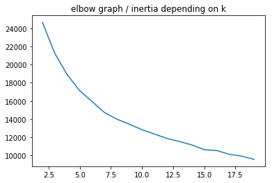
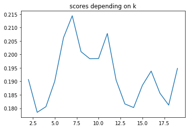
The best nb k of clusters seems to be 7 even if there isn’t any real elbow on the 1st plot.

On the country level

Let’s do exactly the same thing but this same at the country level :

df_solar_transposed = df_solar_co[-24*365*10:].T
plot_elbow_scores(df_solar_transposed, 20)

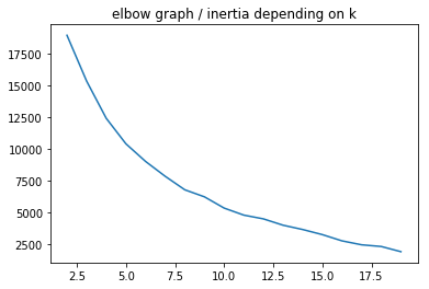
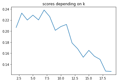
The best nb k of clusters seems to be 6 even if there isn’t any real elbow on the 1st plot.

Finally, we can keep the optimal number k of clusters, and retrieve infos on each group such as number of countries, and names of those countries :

X = df_solar_transposed

km = KMeans(n_clusters=6).fit(X)
X['label'] = km.labels_
print("Cluster nb / Nb of countries in the cluster", X.label.value_counts())

print("\nCountries grouped by cluster")
for k in range(6):
    print(f'\ncluster nb {k} : ', " ".join([country_dict[c] + f' ({c}),' for c in list(X[X.label == k].index)]))

Cluster nb / Nb of countries in the cluster 3    8
1    8
5    4
0    4
2    3
4    2
Name: label, dtype: int64

Countries grouped by cluster

cluster nb 0 :  Estonia (EE), Lithuania (LT), Latvia (LV), Poland (PL),

cluster nb 1 :  Austria (AT), Switzerland (CH), Czech Republic (CZ), Croatia (HR), Hungary (HU), Italy (IT), Slovenia (SI), Slovakia (SK),

cluster nb 2 :  Bulgaria (BG), Greece (EL), Romania (RO),

cluster nb 3 :  Belgium (BE), Germany (DE), Denmark (DK), France (FR), Ireland (IE), Luxembourg (LU), Netherlands (NL), United Kingdom (UK),

cluster nb 4 :  Spain (ES), Portugal (PT),

cluster nb 5 :  Cyprus (CY), Finland (FI), Norway (NO), Sweden (SE),

---

Conclusions

In this first part, we’ve managed to make cluster of countries / regions with similar profiles when it comes to solar generation. This can be convenient when, in the second part, we’ll analyze in depth the data for one country representative of each cluster instead of 30.

References :

• the European Commission’s STETIS program
• Hands-On Unsupervised Learning Using Python
• Towards Data Science