Clustering data containing mixed types with k-prototypes

11 minute read

Image taken from a photo by Ray Hennessy on Unsplash.com.

Introduction

Clustering is grouping objects based on similarities (according to some defined criteria). It can be used in many areas: customer segmentation, computer graphics, pattern recognition, image analysis, information retrieval, bioinformatics, and data compression…

The k-means algorithm is well known for its efficiency in clustering large data sets. However, working only on numeric values prohibits it from being used to cluster real world data containing categorical values:

One hot encoding is often a bad idea:

it doesn’t always make sense to compute the euclidean distance between points with ohe features
if attributes have hundreds or thousands of categories: this will increase both computational and space costs of the k-means algorithm. An other drawback is that the cluster means, given by real values between 0 and 1, do not indicate the characteristics of the clusters.

One solution is to use:

the k-modes algorithm which enables the clustering of categorical only data in a fashion similar to k-means.
the k-prototypes algorithm, through a combination of the principles of k-means & k-modes can deal with mixed data.

!pip install umap-learn
!pip install lightgbm
!pip install kmodes
!pip install shap
!pip install kmodes
# conda install -c conda-forge kmodes


from google.colab import drive
drive.mount('/content/drive')

Theory

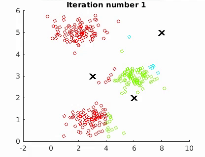
The k-modes algorithm follows the same k-means’ steps

The k-means algorithm

Steps:

Select the Number of Clusters, k
Select k Points at Random
Make k Clusters (by assigning the closest points to the cluster)
Compute New Centroid of Each Cluster
Assess the Quality of Each Cluster (by measuring the Within-Cluster Sum of Squares (WCSS) to quantify the variation within all the clusters)
Repeat Steps 3–5 (with the centroids we calculated previously to make 3 new clusters)

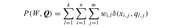
The goal is to minimize the mean of the squared Euclidean distance between the data points and centroids:

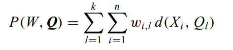
where W is an n × k partition matrix, Q = {Q1, Q2,…, Qk } is a set of k centroids, and d(·, ·) is the distance and X the n data points. The algorithm converges to a local minimum point.
The computational cost of the algorithm is O(Tkn) (T = the iteration number).

The k-modes algorithm

The limitations of k-means can be removed by making the following modifications:

using a simple matching dissimilarity measure for categorical objects,
replacing means of clusters by modes,
using a frequency-based method to find the modes to solve problem

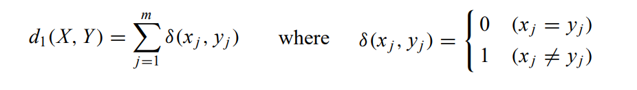
Dissimilarity measure

Often referred to as simple matching “Kaufman and Rousseeuw”, it can be defined by the total mismatches of the corresponding attribute categories of the 2 elements X and Y: the smaller the number of mismatches is, the more similar the 2 elements:

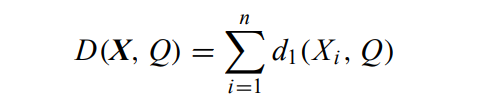
Mode of a set

A mode of X = {X1, X2,…, Xn} is a vector Q = [q1, q2,…, qm] that minimises:

It implies that the mode of a data set X is not unique. For example, the mode of set {[a, b], [a, c], [c, b], [b, c]} can be either [a, b] or [a, c].

The k-modes algorithm

the cost function becomes:

Where m is the number of (categorical) features.
The proof of convergence for this algorithm was not available at the time of the paper’s release. However, its practical use has shown that it always converges. Like the k-means, the k-modes algorithm also produces locally optimal solutions that are dependent on the initial modes and the order of objects (rows) in the data set.

The k-prototypes algorithm

The dissimilarity between two mixed-type objects X and Y:

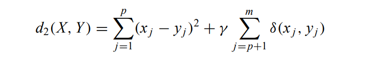
where the first term is the squared Euclidean distance measure on the numeric attributes and the second term is the simple matching dissimilarity measure on the categorical attributes. The weight γ is used to avoid favouring either type of attribute.

the cost function becomes:

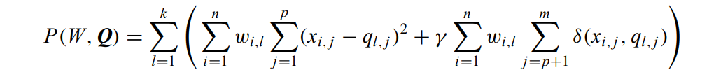
The 2 terms are nonnegative, minimising the total is equivalent to minimising both of them.

Clustering performance

Experiments have shown good results on both synthetic and real world datasets.
It was designed in order to be able to scale but it was more than 20 years ago ! The k-modes and k-prototypes implementations both offer support for multiprocessing via the joblib library, similar to e.g. scikit-learn’s implementation of k-means, using the n_jobs. But it doesn’t seem to be parallelized on multiple nodes: there is an unofficial implementation on PySpark…
An important observation was that the k-modes algorithm was much faster than the k-prototypes algorithm. The key reason is that the k-modes algorithm needs many less iterations to converge than the k-prototypes algorithm because of its discrete nature.

Conclusion

Pros:
- k-modes & k-prototypes can deal with categorical features
- they are scalable & efficient
- k-modes allows missing values and can deal with outliers whereas K-prototypes do not allow numeric attributes to have missing values & is still sensitive to numeric outliers.
Cons:
- the weight γ adds an additional problem: the average standard deviation of numeric attributes is suggested by the author but the user’s knowledge is important in specifying γ: if one thinks should be favoured on numeric attributes (small γ) or categorical ones (large γ).
- the dissimilarity measure makes a separation between categorical & numerical features
Unchanged:
- we still face the common problem: how many clusters are in the data?
- how to initialize the centroids? prefer the init='Cao' by default (based on density / DBSCAN) over ‘Huang’ or ‘random’ which are less efficient. All algorithms are sensitive to the order of observations: it is worth to run it several times, shuffling data in between, averaging resulting clusters and running final evaluations with those averaged clusters centers as starting points
- standardization of numerical features is still required (except in you want to weight features or in special cases: geospacial datas, keeping the same units…)
- Validation of clustering results in case of lack of a priori knowledge to the data: use visualisation techniques
- No ‘silhouette’ implemented / found for the consistency interpretation with dissimilarity metrics.

In practice

import pandas as pd
import numpy as np

from kmodes.kprototypes import KPrototypes

import warnings
warnings.filterwarnings('ignore', category = FutureWarning)
pd.set_option('display.float_format', lambda x: '%.1f' % x)


df = pd.read_csv('/content/drive/MyDrive/kproto/10000 Sales Records.csv')
df.drop(['Country', 'Order Date', 'Order ID', 'Ship Date'], axis=1, inplace=True)
print(df.shape)
df.head()

(10000, 10)

	Region	Item Type	Sales Channel	Order Priority	Units Sold	Unit Price	Unit Cost	Total Revenue	Total Cost	Total Profit
0	Sub-Saharan Africa	Office Supplies	Online	L	4484	651.2	525.0	2920025.6	2353920.6	566105.0
1	Europe	Beverages	Online	C	1075	47.5	31.8	51008.8	34174.2	16834.5
2	Middle East and North Africa	Vegetables	Offline	C	6515	154.1	90.9	1003700.9	592408.9	411292.0
3	Sub-Saharan Africa	Household	Online	C	7683	668.3	502.5	5134318.4	3861014.8	1273303.6
4	Europe	Beverages	Online	C	3491	47.5	31.8	165648.0	110978.9	54669.1

df.select_dtypes('object').nunique()

Region             7
Item Type         12
Sales Channel      2
Order Priority     4
dtype: int64

df.isna().sum()

Region            0
Item Type         0
Sales Channel     0
Order Priority    0
Units Sold        0
Unit Price        0
Unit Cost         0
Total Revenue     0
Total Cost        0
Total Profit      0
dtype: int64

Get the position of categorical columns

categorical_col_positions = [df.columns.get_loc(col) for col in list(df.select_dtypes('object').columns)]
print('Categorical columns           : {}'.format(list(df.select_dtypes('object').columns)))
print('Categorical columns position  : {}'.format(categorical_col_positions))

Categorical columns           : ['Region', 'Item Type', 'Sales Channel', 'Order Priority']
Categorical columns position  : [0, 1, 2, 3]

Convert dataframe to a numpy matrix (required for k-prototypes)

df_matrix = df.to_numpy()
df_matrix

array([['Sub-Saharan Africa', 'Office Supplies', 'Online', ...,
        2920025.64, 2353920.64, 566105.0],
       ['Europe', 'Beverages', 'Online', ..., 51008.75, 34174.25,
        16834.5],
       ['Middle East and North Africa', 'Vegetables', 'Offline', ...,
        1003700.9, 592408.95, 411291.95],
       ...,
       ['Sub-Saharan Africa', 'Vegetables', 'Offline', ..., 388847.44,
        229507.32, 159340.12],
       ['Sub-Saharan Africa', 'Meat', 'Online', ..., 3672974.34,
        3174991.14, 497983.2],
       ['Asia', 'Snacks', 'Offline', ..., 55081.38, 35175.84, 19905.54]],
      dtype=object)

# Choose optimal K using Elbow method
costs = []
for nb_cluster in range(1, 6):
        kprototype = KPrototypes(n_jobs=-1, n_clusters=nb_cluster, random_state=0)
        kprototype.fit_predict(df_matrix, categorical=categorical_col_positions)
        costs.append(kprototype.cost_)
        print(f'Nb of cluster: {nb_cluster}, cost: {kprototype.cost_}')

Nb of cluster: 1, cost: 3.6016173492135216e+16
Nb of cluster: 2, cost: 9627986092172950.0
Nb of cluster: 3, cost: 4960707512782195.0
Nb of cluster: 4, cost: 2927457054391281.0
Nb of cluster: 5, cost: 1975342819318915.2

Sometimes (e.g for a value of k=6) you gert a ValueError: Clustering algorithm could not initialize. Consider assigning the initial clusters manually.
Surprisingly this a feature, not a bug: kmodes is telling you that what you’re doing likely does not make sense given the data you’re presenting it. And because every data set is different, it’s up to you to figure out why :)

import plotly.express as px

df_cost = pd.DataFrame(list(zip(range(1, 6), costs)), columns=['Nb_clusters', 'Costs'])
px.line(df_cost, x="Nb_clusters", y="Costs", 
        title='Elbow method - Cost depending on k',
        width=700, height=500
       ).show()

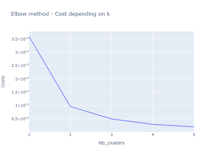
Re-fit the model with the optimal k value

optimal_k = 3
kprototype = KPrototypes(n_jobs=-1, n_clusters=optimal_k, random_state=0)
clusters = kprototype.fit_predict(df_matrix, categorical = categorical_col_positions)
clusters

array([2, 1, 1, ..., 1, 0, 1], dtype=uint16)

model object

kprototype

KPrototypes(gamma=249301.104054418, n_clusters=3, n_jobs=-1, random_state=0)

Cluster centroid

kprototype.cluster_centroids_

array([['7904.365546218487', '593.5265126050414', '457.78549579832264',
        '4622760.54755461', '3559121.1234873924', '1063639.424067227',
        'Europe', 'Household', 'Offline', 'L'],
       ['4046.6694875411376', '163.25910672308513', '105.79686882933991',
        '467709.4517003633', '281142.9546497409', '186566.49705061832',
        'Sub-Saharan Africa', 'Personal Care', 'Online', 'C'],
       ['6093.2754219843555', '384.2645039110791', '275.0975010292268',
        '1995888.1232729559', '1380539.5273034181', '615348.5959695352',
        'Europe', 'Cosmetics', 'Online', 'H']], dtype='<U32')

Check the iteration of the clusters created

kprototype.n_iter_

Assign the cluster label to each record / row

# Add the cluster to the dataframe
df['Cluster Labels'] = kprototype.labels_
df['Segment'] = df['Cluster Labels'].map({0:'First', 1:'Second', 2:'Third'})

# Order the cluster
df['Segment'] = df['Segment'].astype('category')
df['Segment'] = df['Segment'].cat.reorder_categories(['First','Second','Third'])

Cluster interpretation

df.rename(columns = {'Cluster Labels':'Total'}, inplace = True)
df.groupby('Segment').agg(
    {
        'Total':'count',
        'Region': lambda x: x.value_counts().index[0],
        'Item Type': lambda x: x.value_counts().index[0],
        'Sales Channel': lambda x: x.value_counts().index[0],
        'Order Priority': lambda x: x.value_counts().index[0],
        'Units Sold': 'mean',
        'Unit Price': 'mean',
        'Total Revenue': 'mean',
        'Total Cost': 'mean',
        'Total Profit': 'mean'
    }
).reset_index()

	Segment	Total	Region	Item Type	Sales Channel	Order Priority	Units Sold	Unit Price	Total Revenue	Total Cost	Total Profit
0	First	1190	Europe	Household	Offline	L	7904.4	593.5	4622760.5	3559121.1	1063639.4
1	Second	6381	Sub-Saharan Africa	Personal Care	Online	C	4046.7	163.3	467709.5	281143.0	186566.5
2	Third	2429	Europe	Cosmetics	Online	H	6093.3	384.3	1995888.1	1380539.5	615348.6

df_initial = df.copy()
df_initial.drop(columns=['Segment', 'Total'], inplace=True)

Among several clustering methods, which one is the more efficient?

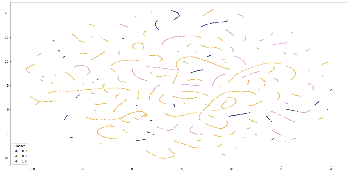
Visualization - UMAP Embedding

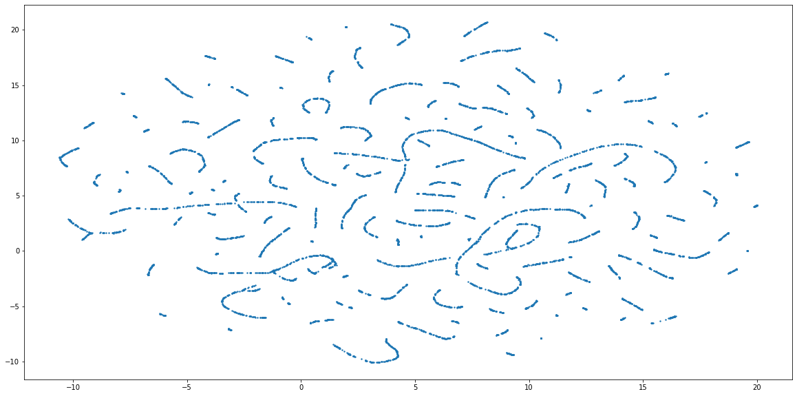
One of the comparison methods will be visual, so we need a way to visulize the quality of clustering. For instance by using the Uniform Manifold Approximation and Projection for Dimension Reduction (UMAP) - a dimensionality reductin technique (like PCA or t-SNE) - to embed the data into 2 dimensions. This will allow to visually see the groups of customers, and how well did the clustering algo do the job. There are 3 steps to get the proper embeddings:

Yeo-Johnson transform the numerical columns & One-Hot-Encode the categorical data
Embed these two column types separately
Combine the two by conditioning the numerical embeddings on the categorical embeddings as suggested here

import umap
from sklearn.preprocessing import PowerTransformer


#Preprocessing numerical
numerical = df_initial.select_dtypes(exclude='object')

for c in numerical.columns:
    pt = PowerTransformer()
    numerical.loc[:, c] = pt.fit_transform(np.array(numerical[c]).reshape(-1, 1))
    
##preprocessing categorical
categorical = df_initial.select_dtypes(include='object')
categorical = pd.get_dummies(categorical)

#Percentage of columns which are categorical is used as weight parameter in embeddings later
categorical_weight = len(df_initial.select_dtypes(include='object').columns) / df_initial.shape[1]

#Embedding numerical & categorical
fit1 = umap.UMAP(metric='l2').fit(numerical)
fit2 = umap.UMAP(metric='dice').fit(categorical)

import matplotlib.pyplot as plt


#Augmenting the numerical embedding with categorical
intersection = umap.umap_.general_simplicial_set_intersection(fit1.graph_, fit2.graph_, weight=categorical_weight)
intersection = umap.umap_.reset_local_connectivity(intersection)
embedding = umap.umap_.simplicial_set_embedding(fit1._raw_data, intersection, fit1.n_components, 
                                                fit1._initial_alpha, fit1._a, fit1._b, 
                                                fit1.repulsion_strength, fit1.negative_sample_rate, 
                                                200, 'random', np.random, fit1.metric, 
                                                fit1._metric_kwds, densmap=False, densmap_kwds={}, output_dens=False)

plt.figure(figsize=(20, 10))
plt.scatter(x=embedding[0][:, 0], y=embedding[0][:, 1], s=2, cmap='Spectral', alpha=1.0)
plt.show()

fig, ax = plt.subplots()
fig.set_size_inches((20, 10))
scatter = ax.scatter(embedding[0][:, 0], embedding[0][:, 1], s=2, c=clusters, cmap='tab20b', alpha=1.0)

# produce a legend with the unique colors from the scatter
legend1 = ax.legend(*scatter.legend_elements(num=optimal_k),
                    loc="lower left", title="Classes")
ax.add_artist(legend1)

Classification evaluation

Another comparison that can be done ib by treating the clusters as labels and building a classification model on top. If the clusters are of high quality, the classification model will be able to predict them with high accuracy. At the same time, the models should use a variety of features to ensure that the clusters are not too simplistic. Overall, I’ll check the quality by:

Distinctivness of clusters by cross-validated F1 score
The informativness of clusters by SHAP feature importances

#Setting the objects to category 
lgbm_data = df.copy()
for c in lgbm_data.select_dtypes(include='object'):
    lgbm_data[c] = lgbm_data[c].astype('category')

from lightgbm import LGBMClassifier
import shap
from sklearn.model_selection import cross_val_score


clf_kp = LGBMClassifier(colsample_by_tree=0.8)
cv_scores_kp = cross_val_score(clf_kp, lgbm_data, clusters, scoring='f1_weighted')
print(f'CV F1 score for K-Prototypes clusters is {np.mean(cv_scores_kp)}')

CV F1 score for K-Prototypes clusters is 1.0

clf_kp.fit(lgbm_data, clusters)

LGBMClassifier(colsample_by_tree=0.8)

explainer_kp = shap.TreeExplainer(clf_kp)
shap_values_kp = explainer_kp.shap_values(lgbm_data)
shap.summary_plot(shap_values_kp, lgbm_data, plot_type="bar", plot_size=(15, 10))

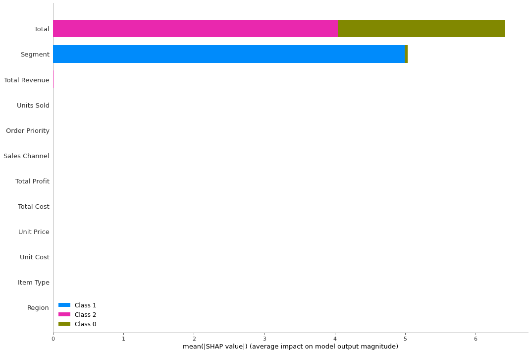
Classifiers for clustering methods that have F1 score close to 1 have produced clusters that are easily distinguishable. Different clustering methods (and classifiers) would probably use more or less features, and some of the categorical features become important. The more features used, the more informative is the clustering algorithm.

Alternative solutions to consider

k-Mediods
- similar to k-means also partitional (breaking the dataset up into groups) and attempt to minimize the distance between points & clusters’ centers
- in contrast to the k-means algo, k-mediods chooses actual data points as centers (mediods or exemplars) for a greater interpretability
- furthermore, k-mediods can be used with arbitrary dissimilarity measures such as Gower, where as k-means generally requires Euclidean distance for efficient solutions
- minimizes a sum of pairwise dissimilarities instead of a sum of squared Euclidean distances
- more robust to noise and outliers than k-means.
Dimensionality Reduction
- to transform our data into a lower dimensional space while retaining as much info as possible or to homogenize our mixed dataset
- tow different techniques:
  - Factorial analysis of Mixed Data - FAMD (a king of PCA on OHE categorical variables & standardize the numerical ones)
  - UMAP as seen above (prediction upon manifold learning & ideas from topological data analysis).

References:

Papers:
- k-modes [HUANG97] [HUANG98]
- k-modes with initialization based on density [CAO09]
- k-prototypes [HUANG97]
Implementations in python (interface similar to scikit-learn): Nico de Vos’ github repo
Examples of use cases:
Other ressources:

I’ve also found a great article covering other clustering models by Advancinganalytics.co.uk

Twitter Facebook LinkedIn

Olivier Brunet