
Neural nets for playing the game of Go
Banner maded from an image by Deepmind on Pexels.com
INTRODUCTION
Objective
The goal of this project is to train several neural networks for playing the game of Go, and to find the most performant architecture. This challenge was proposed by Professor Tristan Cazenave (LAMSADE & Chair AI Advanced of PRAIRIE) during his Deep Learning course, part of the Master IASD at Paris-Dauphine - PSL.
Game of Go
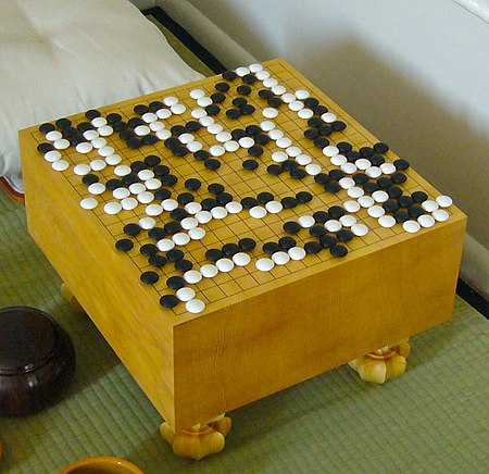
Go is an abstract strategy board game for two players in which the aim is to surround more territory than the opponent. The game was invented in China more than 2,500 years ago and is believed to be the oldest board game continuously played to the present day. […] There are over […] 20 million current players, the majority of whom live in East Asia. [01]
Rules:
The playing pieces are called stones. One player uses the white stones and the other black. The players take turns placing the stones on the vacant intersections (points) on a board. Once placed on the board, stones may not be moved, but stones are removed from the board if the stone (or group of stones) is surrounded by opposing stones on all orthogonally adjacent points, in which case the stone or group is captured. The game proceeds until neither player wishes to make another move. When a game concludes, the winner is determined by counting each player’s surrounded territory along with captured stones and komi (points added to the score of the player with the white stones as compensation for playing second). Games may also be terminated by resignation.
AlphaGo versus Lee Sedol
In March 2016, Seoul, South Korea, a match took place between AlphaGo and Lee Sedol. AlphaGo was developed by Google DeepMind, it uses a combination of machine learning and tree search techniques, combined with extensive training, both from human and computer play. Lee Sedol is widely considered to be one of the greatest player of the past decade, he has won 18 world titles.
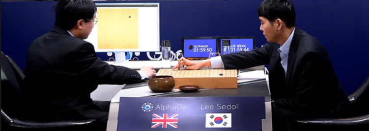
Contrary to expectations, AlphaGo played a number of highly innovative moves which contradicted centuries of received Go knowledge and finally win 4-1 [02]. Later, several improvements were made based on reinforcement learning models: AlphaGo Zero, AlphaZero…
The Dataset
The data used for training comes from the Katago program self played games. KataGo is one of the strongest open-source self-play-trained Go engine, with many improvements to accelerate learning. The dataset we’re going to use is built of 1,000,000 different games in total for the training split (depending on a random state i.e. one random board position). The games of the validation set are never used during training.
KataGo plays Go at a much better level than ELF and Leela, therefore, the networks are trained with better data and provides better results. The input data is composed of 31 19x19 planes (color to play, ladders, current state on two planes, two previous states on multiple planes).
Rules
- In order to be fair about training ressources, the number of networks’ parameters must be lower than 100 000.
- It should use Tensorflow 2.9 & Keras.
- An example of a CNN with two heads is provided in file
golois.py(see next chapter). - The trained networks should also have the same policy & value heads and be
saved in h5 format.
Tournaments:
- Frequently, challengers have to upload their models, and a tournament is organized between them.
- It is a round robin tournament: each contestant meets every other participant. It then return the results / rankings.
- Each network will be used by a PUCT engine that takes 2 seconds of CPU time at each move to play in the tournament.
Objectives
Training deep neural networks and performing tree search are the two pillars of current board games programs. This is also true for the Game of Go. Using a network with two heads instead of two networks was reported to bring significant ELO improvement, the choice of the NN architecture can also lead to many ELO improvement.
Output / Metrics:
- The policy (a vector of size 361 with 1.0 for the move played, 0.0 for the other moves) head is evaluated with the accuracy of predicting the moves of the games
- The value (between 0.0 and 1.0 given by the Monte-Carlo Tree Search representing the probability for White to win) head is evaluated with the Mean Squared Error (MSE) on the predictions of the outcomes of the games.
BASELINE - USUAL CNN
Please refer to the notebook attached named v01_BASELINE_CNN_more_epochs_dataviz.ipynb, comments for most of the lines of code are provided to ease understanding.
Explanation of the code
Constants:
- planes = 31 # each plane corresponds to the properties of a specific game of go
- moves = 361 # number of possible moves in the board (= 19 x 19)
- N = 10000 # number of situations considered in a game
That’s why input_data.shape = (10000, 19, 19, 31)
Variables:
- policy: best shot / move to 1 (–> accurary)
- value: probability for the white to win (between 0 and 1)
- end: position at the end of the game
- group: put connected stones together.
Train & valiation:
At each epoch input_data, value, end, groups are changed:
- first by the
getBatchfunction in order to get data for the training part (see the model.fit(…)) in a deterministic way (reproducible) - then by the
getValidationfunction to assess the model performance on a validation data set (see the model.evaluate(…)). ObviouslygetValidationwill return data that the model hasn’t seen. A shuffle is made at the beginning, so that the timeline is not preserved. Consequently, the RNN architecture (LSTM, GRU and so on…) is not adequate.
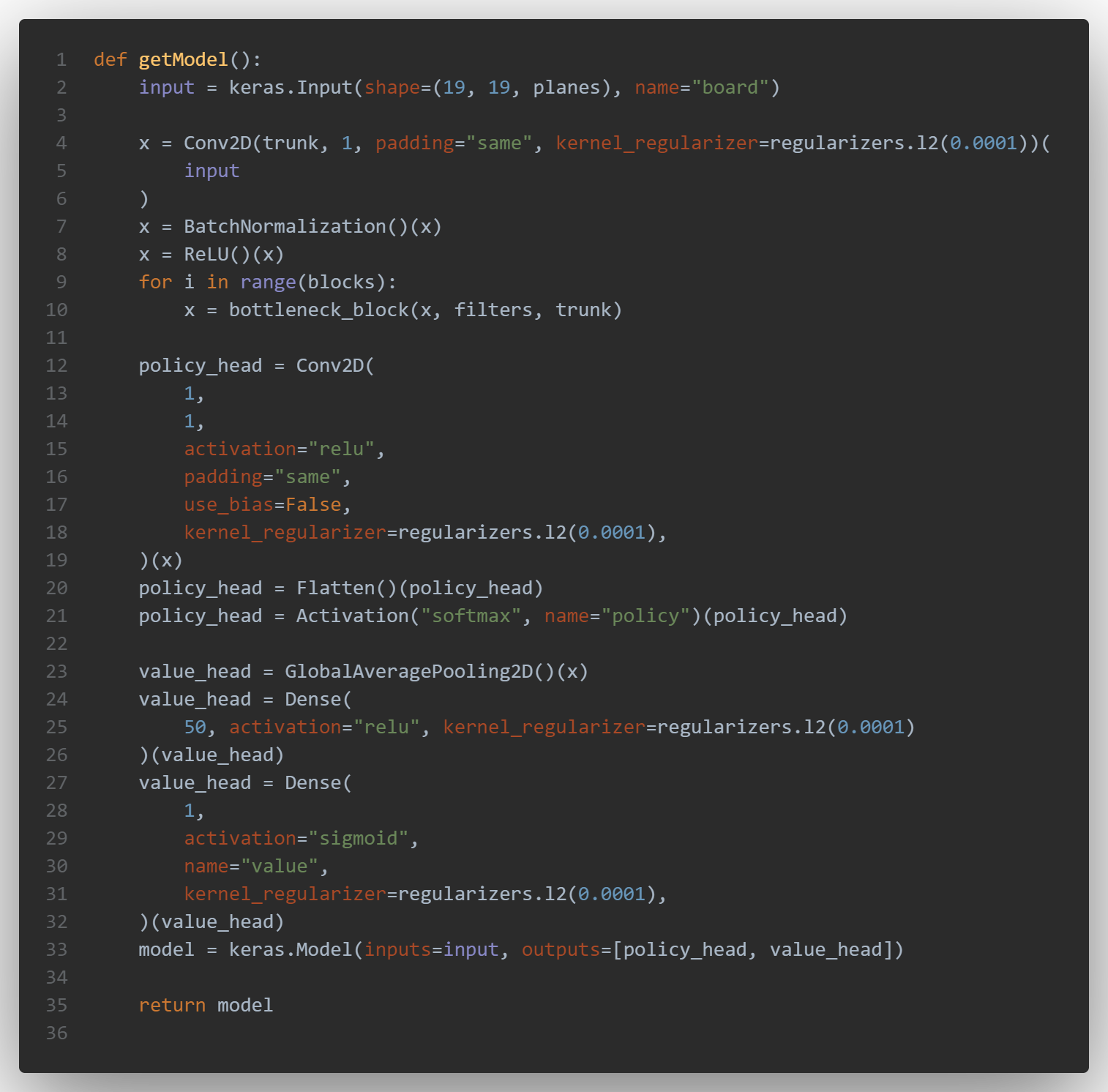
CNN architecture:
Classically, CNN for Go have more than one head. At least, these networks use a policy head, to prescribe moves, and a value head, to evaluate the board quality in terms of future incomes. This output configuration has been popularized by the groundbreaking AlphaZero. 07
The baseline model uses 5 common convolution layers. Then each of the two heads (for the value or the policy) are composed of a convolution layer, a flatten one and - for the value - 2 denses layers:
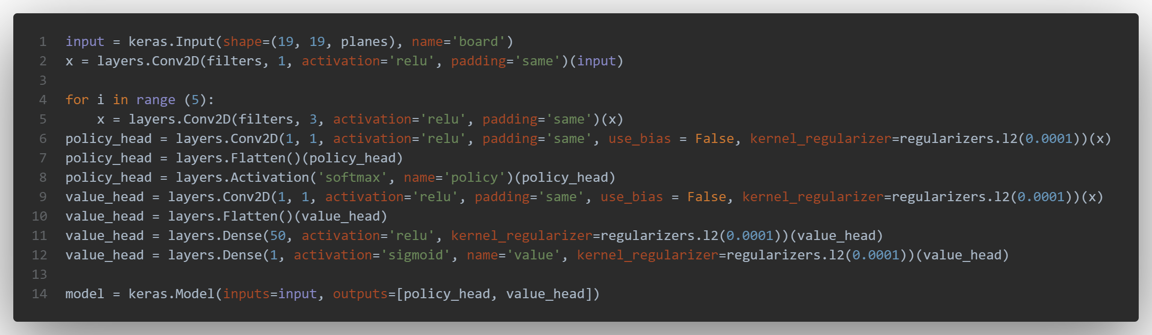
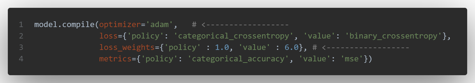
then the compilation is done with the following parameters:
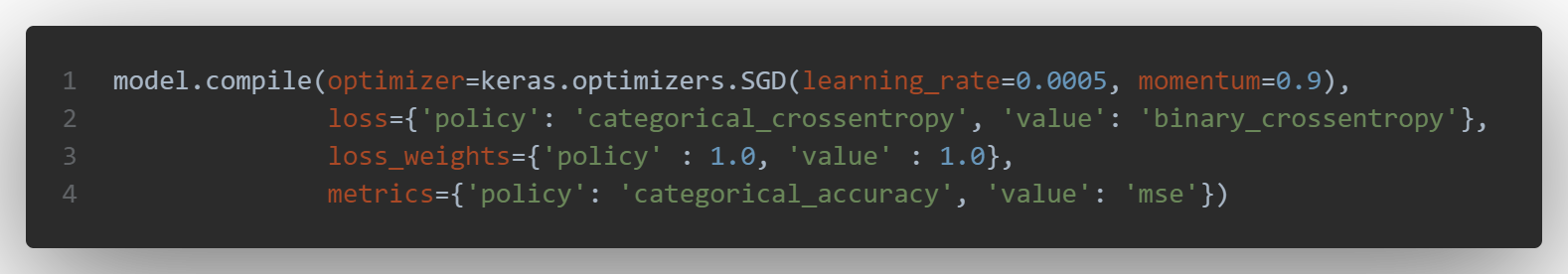
- epochs = 30
- batch = 128
- filters = 32
Results
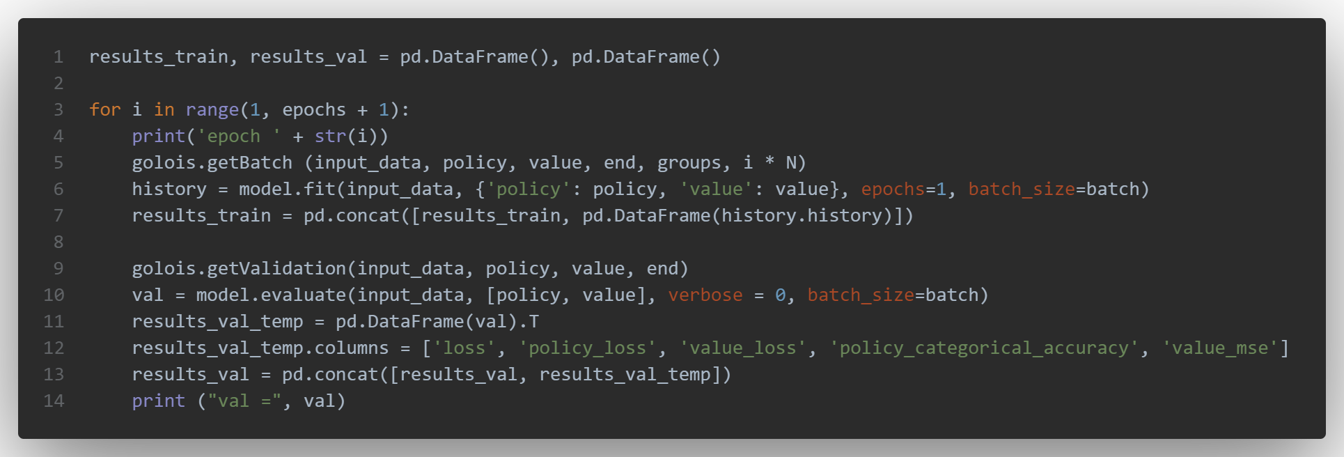
Side note: here, unlike most common code with keras, we’ve created a loop for multiple epochs in order to call each time getBatch and getValidation. As a side effect the history is not saved.
I’ve changed / tweaked a little bit the for loop for the different epochs, so that we can evaluate the model after each fit() call (it’ll also take more time), results are kepts in two pandas dataframes for the train and validation parts:
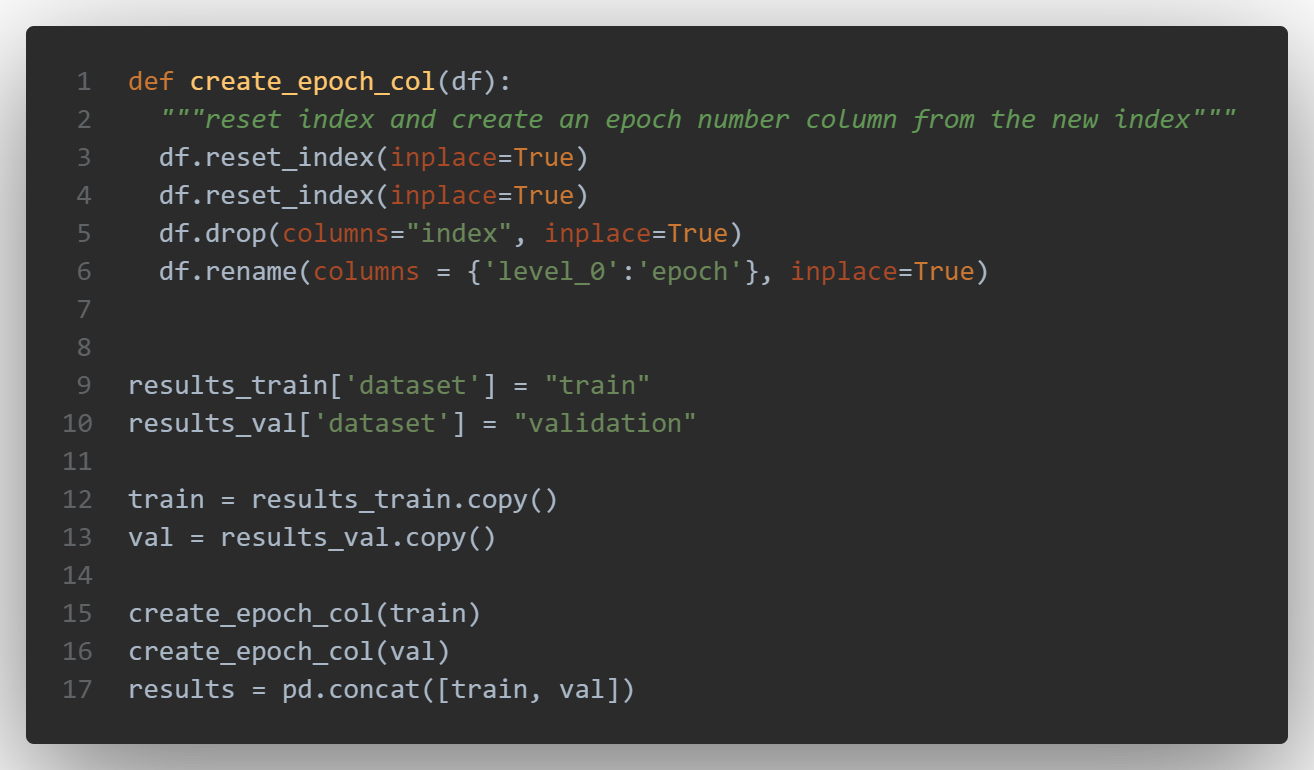
With the following code, you can concatenate all the results of the various epochs:
and then plot the metrics:
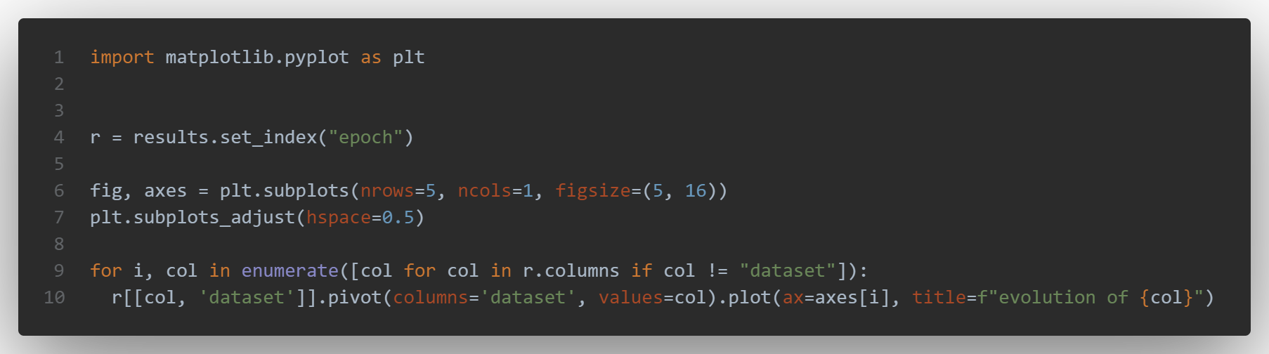
You can see the results below:
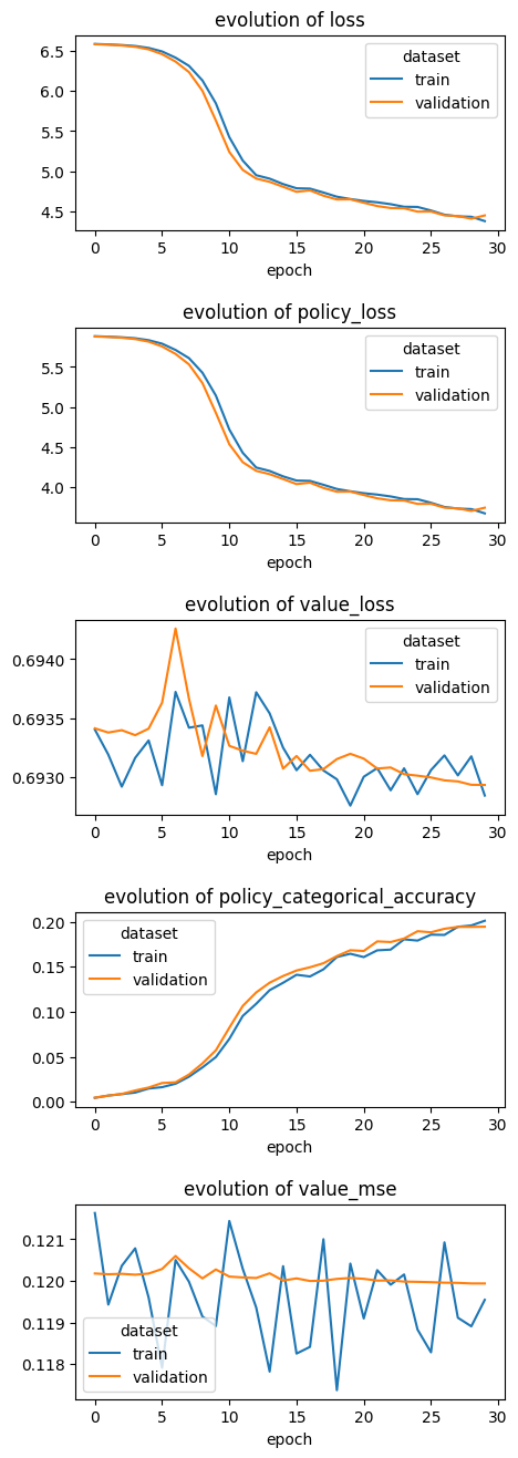
Results:
train - loss: 4.37, policy_loss: 3.67 - value_loss: 0.69 - policy_categorical_accuracy: 0.20 - value_mse: 0.11
valid - loss: 4.44, policy_loss: 3.74 - value_loss: 0.69 - policy_categorical_accuracy: 0.19 - value_mse: 0.11
Overfitting vs underfitting
The metrics on the validation dataset follow closely the ones on the train set, thus the model isn’t overfitting. Consequently we don’t have to use DropOut, Data augmentation (such as flipping images…) or early_stopping strategies so that the model would generalize better. On the other hand, we aren’t sure that the model is not underfitting, because more complex models would probably perform better: let’s discuss the potential improvement we can make.
Potential improvements
- With classical CNN there is an issue with vanishing gradient:
When there are more layers in the network, the value of the product of derivative decreases until at some point the partial derivative of the loss function approaches a value close to zero, and the partial derivative vanishes.
With shallow networks, sigmoid function can be used as the small value of gradient does not become an issue. When it comes to deep networks, the vanishing gradient could have a significant impact on performance. The weights of the network remain unchanged as the derivative vanishes. During back propagation, a neural network learns by updating its weights and biases to reduce the loss function. In a network with vanishing gradient, the weights cannot be updated, so the network cannot learn. The performance of the network will decrease as a result. [03]
This is also demonstrated practically this paper [07]: non-linearity plays an important role in neural network. Without them, they lose their expressiveness power. It also has an important impact on the neural net training. In particular, the activation shape the derivatives of the network
Changing the activation function could be a solution, for instance the Swish function - proposed by Google - could be an alternative to the sigmoid function. It performs better than ReLU in the case of deeper neural networks, it allows data normalization and leads to quicker convergence and learning of the NN. Swish can work around and prevent the vanishing gradient program, and hence allow training for small gradient updates. Anyway it has some limitations: it is time-intensive to compute for deeper layers with large parameter dimensions.
- Using other architecture is an other way to get better results, some of them may act as a workaround for the vanishing gradient issue.
- A better optimizer or an adaptation of the learning through the epochs, in order to converge more rapidly and to try as musch as possible to avoid local minimums.
- We can also consider different weights between the two head’s metrics.
The later ideas will be used in the following chapters. For example with the same CNN, if we only change the activation function to swish and train the model during 240 epochs, the results get better:
train - loss: 3.74 - policy_loss: 3.04 - value_loss: 0.69 - policy_categorical_accuracy: 0.30 - value_mse: 0.11
valid - loss: 3.73 - policy_loss: 3.03 - value_loss: 0.69 - policy_categorical_accuracy: 0.30 - value_mse: 0.11
The policy accuracy has increased from 0.2 to 0.3.
SHUFFLENET
ShuffleNet is a CNN designed specially for mobile devices with very limited computing power. The architecture utilizes two new operations, pointwise group convolution and channel shuffle, to reduce computation cost while maintaining accuracy.
How the ShuffleNet works ? [08]
- Channel Shuffle for Group Convolutions
Xception and ResNeXt balance anexcellent trade-off between representation capability and computational cost, by introducingdepthwise separable convolutions or group convolutionsinto the building blocks, but cannot fully take the 1x1 convolutions, called pointwise convolutions, into account. In tiny networks, expensive pointwise convolutions result in limited number of channels to meet the complexity constraint, which might significantly damage accuracy.
Let’s compare 3 different cases relative to colored picture with 3 channels (RGB):
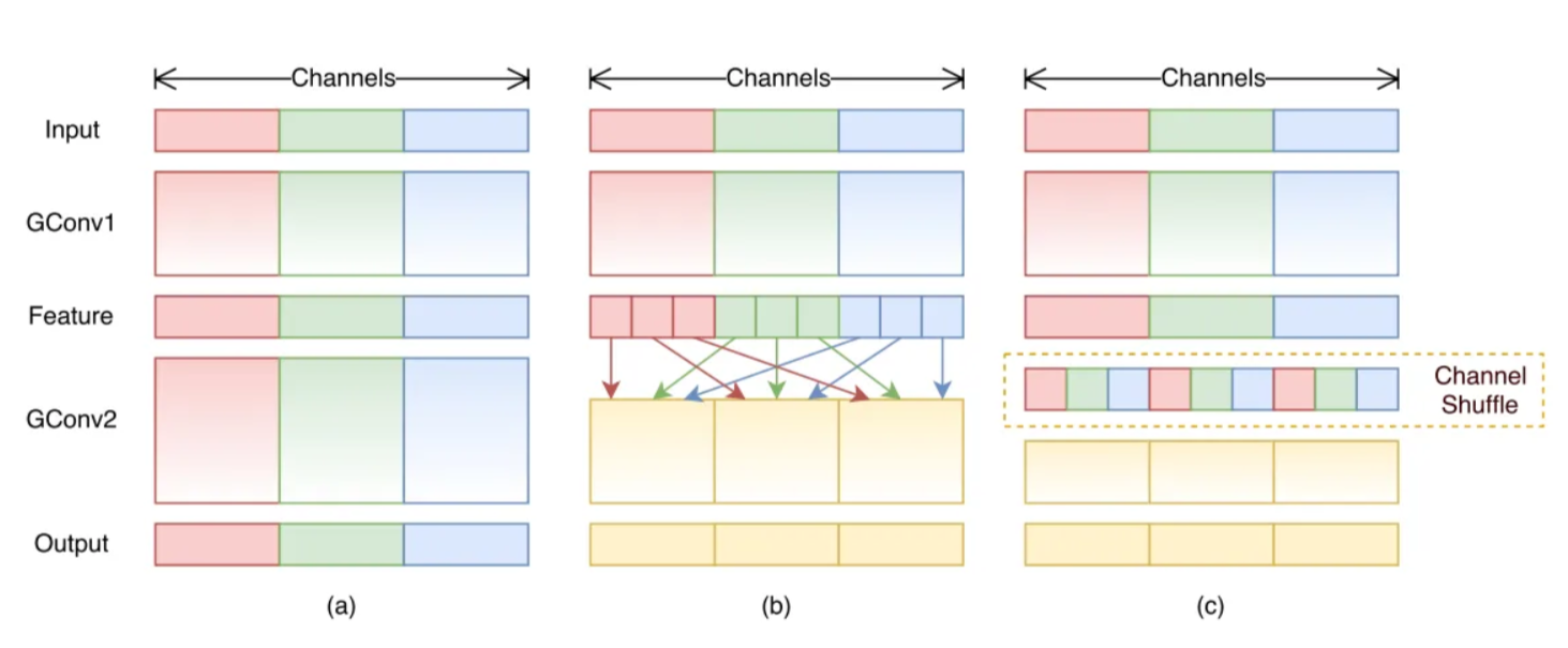
Figure 1(a) illustrates a situation of two stacked group convolution layers, which has twofold properties, blocking the information flow between channel groups and weakening representations.
Figure 1(b) shows that the group convolution is allowed to obtain input data from different groups. Notice that the input channels are fully related to the output ones.
Figure 1(c) sets up the feature map from the previous group layer, which is then implemented by a channel shuffle operation. Channel shuffle operation is able to construct more powerful structures with multiple group convolutional layers.
The configuration in Figure 1(c) is preferable, because the channel shuffle operation still applies in the stacked layers, though the convolutions in Figure 1(b) have different number of groups. Additionally, it is differentiable so it is embedded into network structures.
- ShuffleNet Unit
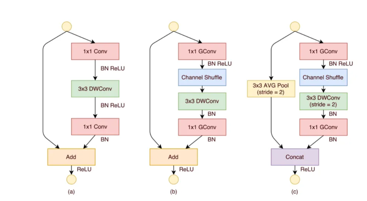
Figure 2(a) is a bottleneck unit with depthwise convolution (3x3 DWConv).
Figure 2(b) is a ShuffleNet unit with pointwise group convolution and channel shuffle.
The purpose of the second pointwise group convolution is to recover the channel dimension to match the shortcut path.
Figure 2(c) is a ShuffleNet unit with stride of 2.
Because of the pointwise group convolution with channel shuffle, all components in ShuffleNet unit can be computed efficiently.
Implementation
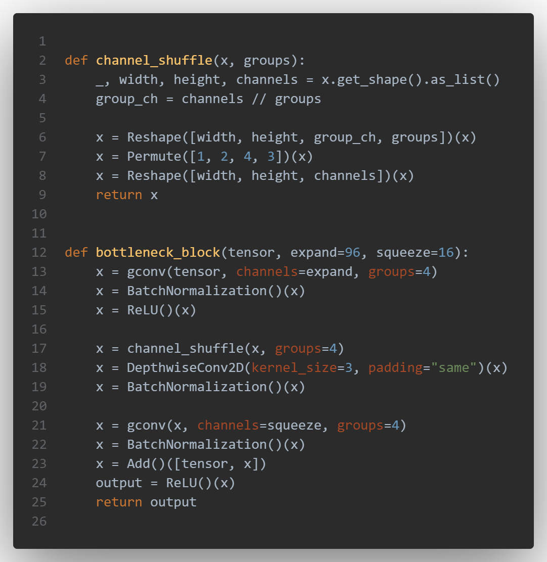
Here is the code used for the model version 12, it starts with a Conv2D, followed by several blocks of bottleneck:
The main branch of the block consists of:
- line 13: 1×1 Group Convolution with 1/6 filters followed by Batch Normalization and ReLU
- line 17: Channel Shuffle
- line 18: 3×3 DepthWise Convolution followed by Batch Normalization
- line 21: 1×1 Group Convolution followed by Batch Normalization
The tensors of the main branch and the shortcut connection are then concatenated and a ReLU activation is applied to the output.
Results
- Total params: 28,485
- Trainable params: 24,581
- Non-trainable params: 3,904
train - loss: 6.58 - policy_loss: 5.88 - value_loss: 0.68 - policy_categorical_accuracy: 0.003 - value_mse: 0.11
valid - loss: 6.58 - policy_loss: 5.88 - value_loss: 0.68 - policy_categorical_accuracy: 0.003 - value_mse: 0.11
The results are not good, the accuracy is really low: it’s a little bit disappointing, but I should have tried multiple shufflenet architectures. It could have also been interesting to use the Adam optimizer to compare to the default choice.
RESNET
How the ResNet works ?
The use of residual networks can improve the training of a policy network. Training is faster than with usual CNN & residual networks achieve a relatively high accuracy on the test set. The principle of residual nets is to add the input of the layer to the output of each layer. With this simple modification training is faster and enables deeper networks:
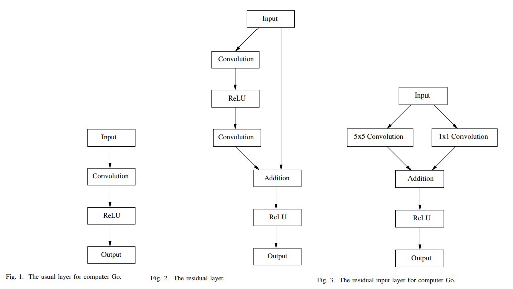
The usual layer used in computer Go program such as AlphaGo is composed of a convolutional layer and of a ReLU layer as shown in figure above. The residual layer used for image classification adds the input of the layer to the output of the layer. 04
How exactly could this prevent the vanishing gradient problem (VGP)?
Initially ResNets were not introduced to specifically solve the VGP, but to improve learning in general. The authors of ResNet, in the original paper, noticed that NN without residual connections don’t learn as well as ResNets, although they are using batch normalization, which, in theory, ensures that gradients should not vanish. But ResNets may also potentially mitigate (or prevent to some extent) the VGP:
The skip connections allow information to skip layers, so, in the forward pass, information from layer l can directly be fed into layer l+t (i.e. the activations of layer l are added to the activations of layer l+t), for t≥2, and, during the forward pass, the gradients can also flow unchanged from layer l+t to layer l.
The VGP occurs when the elements of the gradient (the partial derivatives with respect to the parameters of the NN) become exponentially small, so that the update of the parameters with the gradient becomes almost insignificant (i.e. if you add a very small number 0<ϵ≪1 to another number d, d+ϵ is almost the same as d) and, consequently, the NN learns very slowly or not at all. Given that these partial derivatives are computed with the chain rule, this can easily occur, because you keep on multiplying small (finite-precision) numbers.
The deeper the NN, the more likely the VGP can occur. The addition of the information from layer l will make the activations bigger, thus, to some extent, they will prevent these activations from becoming exponentially small. A similar thing can be said for the back-propagation of the gradient. (source StackExchange)
Implementation
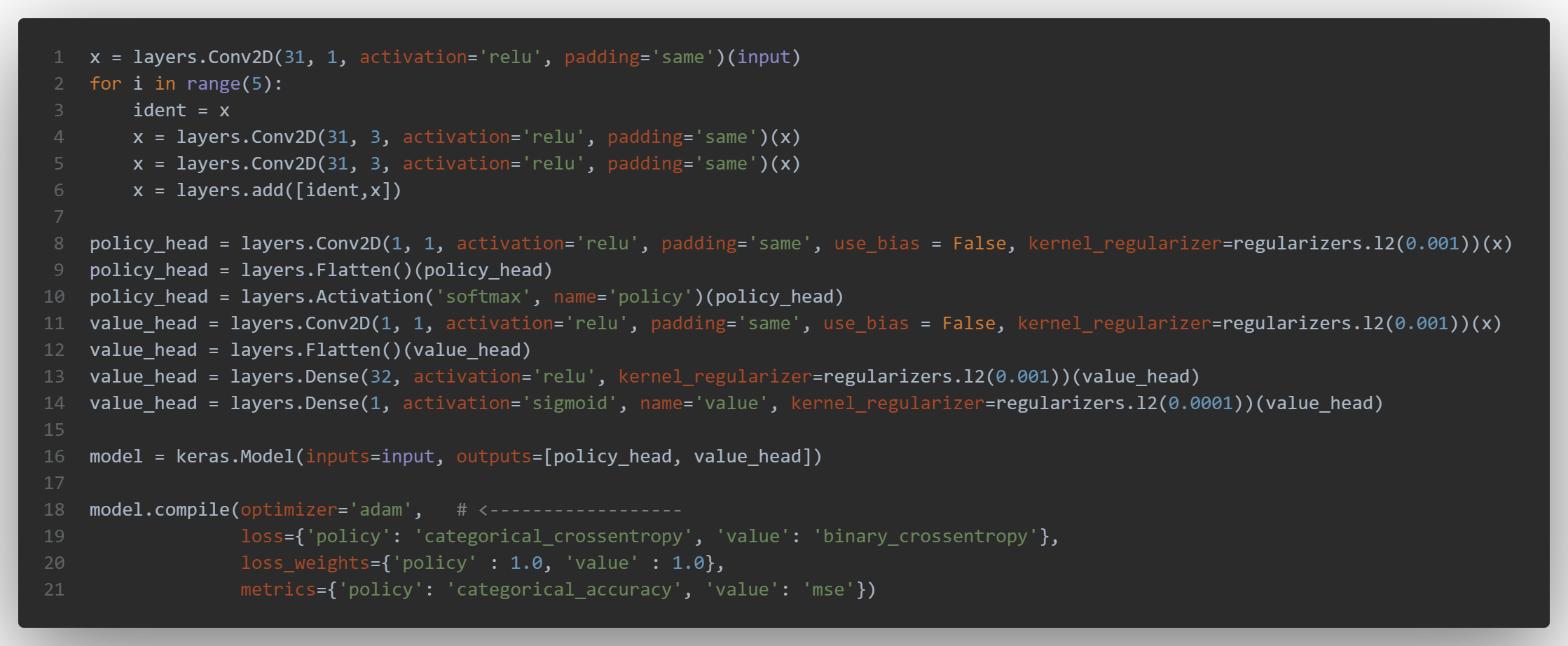
Here is the code of version 17: unfortunately i’ve not uploaded the h5 on the google drive in order to be part of the tournament!
The addition is made line 6, with the variable “ident” initialized with the value of x before the 2 convolutions:
Results
- Total params: 99,471
- Trainable params: 99,471
- Non-trainable params: 0
train - loss: 3.22 - policy_loss: 2.53 - value_loss: 0.69 - policy_categorical_accuracy: 0.37 - value_mse: 0.11
valid - loss: 3.24 - policy_loss: 2.55 - value_loss: 0.69 - policy_categorical_accuracy: 0.37 - value_mse: 0.11
The results are quite promissing: the accuracy is good. Here, the use of the Adam optimizer was a “game changer”, because the accuracy was “only” 0.31 with SGD.
What is Adam?
Adam optimization - first presented as a conference paper at ICLR 2015 - is an extension to Stochastic gradient decent and can be used in place of classical SGD to update network weights more efficiently. Adam uses Momentum and Adaptive Learning Rates to converge faster.
- Momentum
When explaining momentum, researchers and practitioners alike prefer to use the analogy of a ball rolling down a hill that rolls faster toward the local minima, but essentially what we must know is that the momentum algorithm, accelerates stochastic gradient descent in the relevant direction, as well as dampening oscillations.
- Adaptive Learning Rate
Adaptive learning rates can be thought of as adjustments to the learning rate in the training phase by reducing the learning rate to a pre-defined schedule. In keras, one can change the “decay” value for that purpose.
Imagine a ball, we started from some point and then the ball goes in the direction of downhill or descent. If the ball has the sufficient momentum than the ball will escape from the well or local minima in our cost function graph.
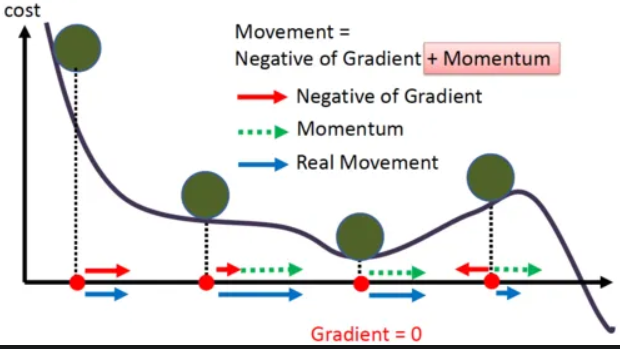
Gradient Descent with Momentum considers the past gradients to smooth out the update. It computes an exponentially weighted average of your gradients, and then use that gradient to update the weights.
MOBILENET
How the MobileNet works?
MobileNet and then MobileNetV2 are parameter efficient NN architectures for computer vision. Instead of usual convolutional layers in the block they use depthwise convolutions. They also use 1x1 filters to pass from a small number of channels in the trunk to 6 times more channels in the block.
Mobile Networks are commonly used in computer vision to classify images. They obtain high accuracy for standard computer vision datasets while keeping the number of parameters relatively lower than other neural networks architectures.
The proposed MobileNetV2 network architecture (for an other task / purpose):
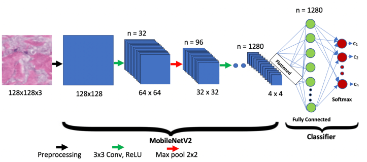
[…] The principle of MobileNetV2 is to have blocks as in residual networks where the input of a block is added to its output. But instead of usual convolutional layers in the block they use depthwise convolutions. Moreover the number of channels at the input and the output of the blocks (in the trunk) is much smaller than the number of channels for the depthwise convolutions in the block. In order to efficiently pass from a small number of channels in the trunk to a greater number in the block, usual convolutions with cheap 1x1 filters are used at the entry of the block and at its output. […]
There is a trade-off between the accuracy and the speed of the networks. Some experiments were made and explained in this paper [05] with various depth and width settings of networks: when increasing the size of the networks there is a balance to keep between the depth and the width of the networks:
[…] to improve the performance of a network it is better to make both the number of blocks (i.e. the depth of the network) and the number of planes (i.e. the width of the network) grow together. […]
Implementation
Here is the code of version 21, with the depthwise convolution line 5:
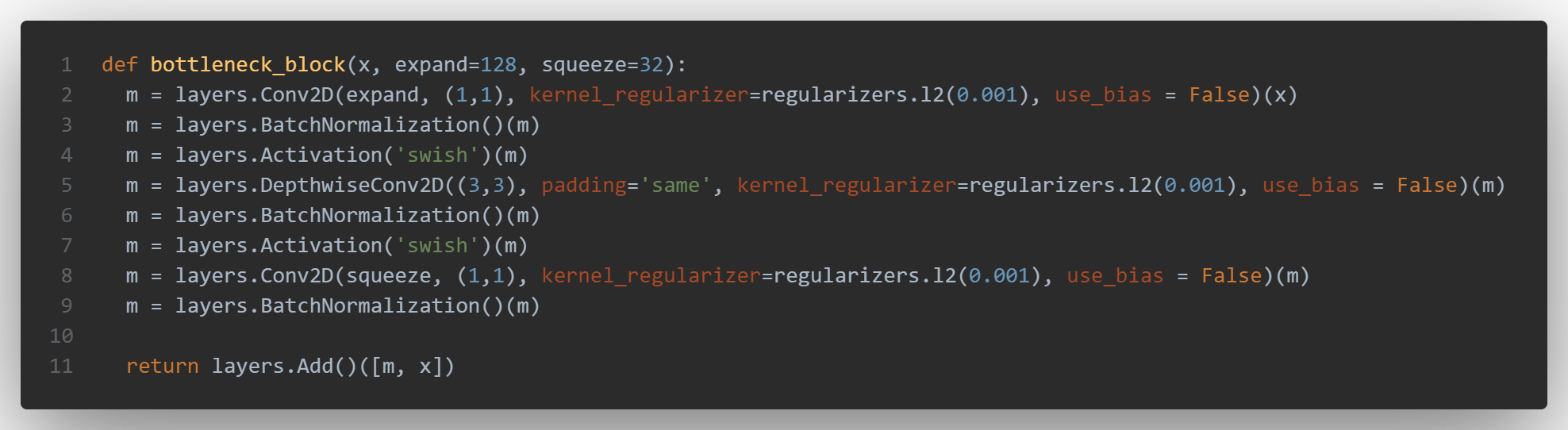
we can see the the “bottleneck_block” function called several times in a loop before the two heads, which are unchanged:
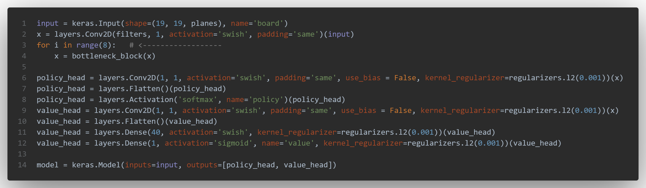
several tries were made with different loss_weights:
Results
- Total params: 99,577
- Trainable params: 94,969
- Non-trainable params: 4,608
train - loss: 6.10 - policy_loss: 2.24 - value_loss: 0.61 - policy_categorical_accuracy: 0.42 - value_mse: 0.09
valid - loss: 6.14 - policy_loss: 2.23 - value_loss: 0.62 - policy_categorical_accuracy: 0.42 - value_mse: 0.08
Only the change of weight for losses managed to decrease the value mean squared error, otherwise the policy accuracy still remains the highest values i could get.
CONCLUSION
Results comparison
The table below summarises all the differents architectures tried for this project. That way, we can see the influence of a specific parameter between two version’s results. The models used for the tournament are selected in green. Unfortunately, the version 17 was not uploaded:
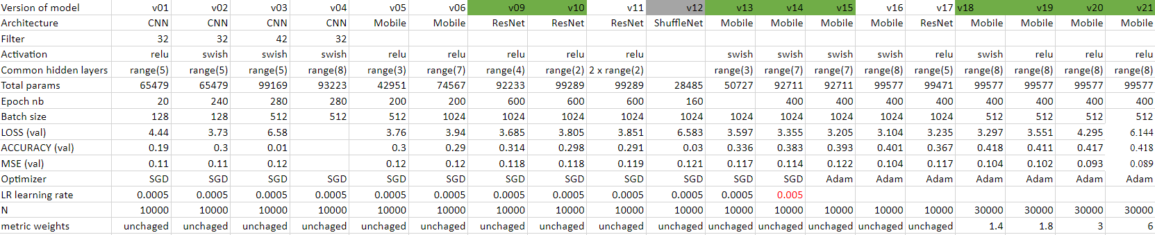
Strategy
- i sould have tried more versions of shufflenet but at that moment, other architectures seem to be more efficient.
- at first, i focused on increasing the accuracy, because the MSE of the value didn’t change that much.
- i’ve changed parameters one by one between versions in order to see its impact and try to modify both depth or width, or both.
- a huge gap in the results was obtained by changing the optimizer.
- the only way to decrease significantly the value’s MSE - at the end - was to change the losses’ weighs, to give more importance on the later for the optimizer because models don’t seem to learn the value.
- the metrics evolution graphs for each model version are not presented here but remains quite the sames: this is especially true for the evolutions of policy loss and of categorical accuracy.
Other solutions
- The keras & tensorflow version installed by default on the SaturnCloud (which provide freely 30 hours of GPU monthly) virtual machine doesn’t allow me to use other optimizers such as LION (release recently by Google Brain) or ADAMW.
- An other solution would be to use Transformers, to my knowledge there is not any ground breaking transformers’ architecture for computer vision yet, but some models might deserve a try.
- We could have; of course; use more deep models but that would leads to more than 100,000 parameters.
- Combining models with Reinforcement Learning is an other option but goes beyond the scope of this study.
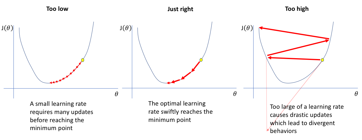
- Learning rate schedules and decay is also to condiser: we can view the process of learning rate scheduling as:
- Finding a set of reasonably “good” weights early in the training process with a larger LR.
- Tuning these weights later in the process to find more optimal weights using a smaller LR.
- or Cosine Annealing [07]: [..] using a different optimization strategy, a neural net can end in a better optimum. [..] this can be achieved by using Stochastic Gradient Descent with warms Restart. In particular, the learning rate is restarted multiple times. This way, the objective landscape is explored further and the best solution of all restart is kept. Furthermore, using a peculiarly aggressive learning rate strategies like cosine annealing can lead to better convergence.
- Whereas Transfer Learning is not suitable here (because of the parameters number limitation), knowledge distillation (the process of transferring knowledge from a large model to a smaller one), on the other hand could be really interesting.
References
- 01 - Game of Go - Wikipedia
- 02 - AlaphaGo - Deepmind
- 03 - Vanishing gradient - kdnuggets
- 04 - Residual Networks for Computer Go, Tristan Cazenave. IEEE Transactions on Games, Vol. 10 (1), pp. 107-110, March 2018
- 05 - Improving Model and Search for Computer Go, Tristan Cazenave. IEEE Conference on Games 2021
- 06 - Mobile Networks for Computer Go, Tristan Cazenave. IEEE Transactions on Games, Vol. 14 (1), pp. 76-84, January 2022
- 07 - Cosine Annealing, Mixnet and Swish Activation for Computer Go, Tristan Cazenave, Julien Sentuc, Mathurin Videau. Advances in Computer Games 2021
- 08 - ShuffleNet: An Extremely Efficient Convolutional Neural Network for Mobile Devices by SyncedReview on Medium
