Pandas - All You Need To Know

I’ve already done the same thing with Numpy, so i’ve decided to create a cheat-sheet for Pandas too :) Most of what you’ll find below is taken from Khalil El Mahrsi’s course that you can find on his website smellydatascience.com published under the Creative Commons Attribution-NonCommercial-ShareAlike 4.0 International Public License (CC BY-NC-SA 4.0). So all the credits goes to him. I’ve added few tips found here and there…

You’ll also found my Anki decks related to Numpy & Pandas on github.

Introduction

• a Python package for tabular data analysis and manipulation
• powerful & intuitive : fast, flexible and easy to use
• open source

Tabular data definition:
data structured into a table (dataframe) ie into rows & columns

• row: entities, objects, observations, instances
• column: variables, features, attibutes

Variable types

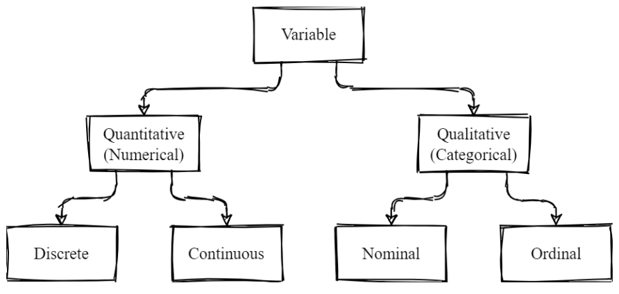
Quantitative (Numerical) Variables

• A quantitative variable has values that are numeric and that reflect a notion of magnitude
• Quantitative variables can be
  • Discrete → finite set of countable values (often integers)
    e.g., number of children per family, number of rooms in a house, …
  • Continuous → infinity of possible values
    e.g., age, height, weight, distance, date and time, …
• Math operations on quantitative variables make sense
  e.g., a person who has 4 children has twice as much children as a person who has 2

Qualitative (Categorical) Variables

• A qualitative variable’s values represent categories (modalities, levels)
• They do not represent quantities or orders of magnitude
• Qualitative variables can be
  • Nominal → modalities are unordered e.g., color,
  • Ordinal → an order exists between modalities e.g., cloth sizes (XS, S, M, L, XL, XXL, …), satisfaction level (very dissatisfied, dissatisfied, neutral, satisfied, very satisfied), …

/!\ Encoding a categorical variable with a numeric data type (e.g., int) does not make it quantitative!

Pandas’ Features

• Based on NumPy → many concepts (indexing, slicing, …) work similarly
• Two main object types
  • DataFrame → 2-dimensional data structure storing data of different types (strings, integers, floats, …) in columns
  • Series → represents a column (series of values)

Installing & importing pandas

!conda install pandas
!pip install pandas

import pandas as pd

Basic Functionalities

dataset used for the below examples: The Bank Marketing Data Set Variables

• age: age in years (numeric)
• job: the customer’s job category (categorical)
• marital:the customer’s marital status (categorical)
• education: the customer’s education level (ordinal)
• default: whether the customer has a loan in default (categorical)
• housing: whether the customer has a housing loan (categorical)
• loan: whether the customer has a presonal loan (categorical)
  …
• y: how the customer responded to a marketing campaign (target variable)

Pandas provides reader and writer functions for handling popular formats: CSV, JSON, parquet, Excel, SQL databases…

reader function to load a data frame from a CSV file

# df = pd.read_csv(file_path, sep=separator,...) 
# default sep = ","
df = pd.read_csv("./bank.csv", sep=';')

df.head()

	age	job	marital	education	default	balance	housing	loan	contact	day	month	duration	campaign	pdays	previous	poutcome	y
0	30	unemployed	married	primary	no	1787	no	no	cellular	19	oct	79	1	-1	0	unknown	no
1	33	services	married	secondary	no	4789	yes	yes	cellular	11	may	220	1	339	4	failure	no
2	35	management	single	tertiary	no	1350	yes	no	cellular	16	apr	185	1	330	1	failure	no
3	30	management	married	tertiary	no	1476	yes	yes	unknown	3	jun	199	4	-1	0	unknown	no
4	59	blue-collar	married	secondary	no	0	yes	no	unknown	5	may	226	1	-1	0	unknown	no

df.to_csv("bank_copy.csv")
#!dir or !ls -alh

view the beginning or the end of a series / dataframe

df.head(2)

	age	job	marital	education	default	balance	housing	loan	contact	day	month	duration	campaign	pdays	previous	poutcome	y
0	30	unemployed	married	primary	no	1787	no	no	cellular	19	oct	79	1	-1	0	unknown	no
1	33	services	married	secondary	no	4789	yes	yes	cellular	11	may	220	1	339	4	failure	no

df.tail(3)

	age	job	marital	education	default	balance	housing	loan	contact	day	month	duration	campaign	pdays	previous	poutcome	y
4518	57	technician	married	secondary	no	295	no	no	cellular	19	aug	151	11	-1	0	unknown	no
4519	28	blue-collar	married	secondary	no	1137	no	no	cellular	6	feb	129	4	211	3	other	no
4520	44	entrepreneur	single	tertiary	no	1136	yes	yes	cellular	3	apr	345	2	249	7	other	no

get the shape of a DataFrame or a Series

• DataFrame → tuple (row_count, column_count)
• Series → singleton tuple (length, )

df.shape

(4521, 17)

The column names of a DataFrame can be accessed using its columns attribute

df.columns

Index(['age', 'job', 'marital', 'education', 'default', 'balance', 'housing',
       'loan', 'contact', 'day', 'month', 'duration', 'campaign', 'pdays',
       'previous', 'poutcome', 'y'],
      dtype='object')

Use the dtypes attribute to check the data types of a Series or a DataFrame’s columns

• pandas mostly relies on NumPy arrays and dtypes (bool, int, float, datetime64[ns], …)
• pandas also extends some NumPy types (CategoricalDtype, DatetimeTZDtype, …)
• Two ways to represent strings: object dtype (default) or StringDtype (recommended)

df.dtypes

age           int64
job          object
marital      object
education    object
default      object
balance       int64
housing      object
loan         object
contact      object
day           int64
month        object
duration      int64
campaign      int64
pdays         int64
previous      int64
poutcome     object
y            object
dtype: object

Technical summary
A technical summary of a DataFrame can be accessed using the info() method. It contains

• The type of the DataFrame
• The row index (RangeIndex in the example) and its number of entries
• The total number of columns
• For each column -The column’s name
  • The count of non-null values
  • The column’s data type
• Column count per data type
• Total memory usage

df.info()

<class 'pandas.core.frame.DataFrame'>
RangeIndex: 4521 entries, 0 to 4520
Data columns (total 17 columns):
 #   Column     Non-Null Count  Dtype 
---  ------     --------------  ----- 
 0   age        4521 non-null   int64 
 1   job        4521 non-null   object
 2   marital    4521 non-null   object
 3   education  4521 non-null   object
 4   default    4521 non-null   object
 5   balance    4521 non-null   int64 
 6   housing    4521 non-null   object
 7   loan       4521 non-null   object
 8   contact    4521 non-null   object
 9   day        4521 non-null   int64 
 10  month      4521 non-null   object
 11  duration   4521 non-null   int64 
 12  campaign   4521 non-null   int64 
 13  pdays      4521 non-null   int64 
 14  previous   4521 non-null   int64 
 15  poutcome   4521 non-null   object
 16  y          4521 non-null   object
dtypes: int64(7), object(10)
memory usage: 600.6+ KB

Statistical Summary of Numerical Columns
Use the describe() method to access a statistical summary (mean, standard deviation, min, max, …) of numerical columns of a DataFrame

# transpose the statistical summary for better readability
df.describe().T

	count	mean	std	min	25%	50%	75%	max
age	4521.0	41.170095	10.576211	19.0	33.0	39.0	49.0	87.0
balance	4521.0	1422.657819	3009.638142	-3313.0	69.0	444.0	1480.0	71188.0
day	4521.0	15.915284	8.247667	1.0	9.0	16.0	21.0	31.0
duration	4521.0	263.961292	259.856633	4.0	104.0	185.0	329.0	3025.0
campaign	4521.0	2.793630	3.109807	1.0	1.0	2.0	3.0	50.0
pdays	4521.0	39.766645	100.121124	-1.0	-1.0	-1.0	-1.0	871.0
previous	4521.0	0.542579	1.693562	0.0	0.0	0.0	0.0	25.0

Value Counts of Qualitative Columns
Use the value_counts() method to count the number of occurrences of each value in a Series (or DataFrame). Use normalize=True in the method call to get percentages

# count occurences of each category of marital
# (can also be used with numerical variables)

df['marital'].value_counts()

married     2797
single      1196
divorced     528
Name: marital, dtype: int64

# percentages instead of counts

df['marital'].value_counts(normalize=True)

married     0.618668
single      0.264543
divorced    0.116788
Name: marital, dtype: float64

# for a DF, value_counts() counts occurences
# of rows (i.e., value combinations)

df[['marital', 'housing']].value_counts()

marital   housing
married   yes        1625
          no         1172
single    yes         636
          no          560
divorced  yes         298
          no          230
dtype: int64

Selecting a Single Column
To select a single column from a DataFrame, specify its name within square brackets → df[col]. The retrieved object is a Series.

jobs = df['job']
type(jobs)

pandas.core.series.Series

jobs.head()

0     unemployed
1       services
2     management
3     management
4    blue-collar
Name: job, dtype: object

Selecting Multiple Columns
To select multiple columns, provide a list of column names within square brackets → df[[col_1, col_2, …]]. The retrieved object is a DataFrame

df[['age', 'education', 'job', 'loan']].head()

	age	education	job	loan
0	30	primary	unemployed	no
1	33	secondary	services	yes
2	35	tertiary	management	no
3	30	tertiary	management	yes
4	59	secondary	blue-collar	no

Dropping Columns
Instead of selecting columns, you can drop unwanted columns using the drop() method. Be sure to specify axis=1 (otherwise, will attempt to drop rows) To modify the original data frame, use inplace=True in the method call

df_with_cols_dropped = df.drop(['balance', 'day', 'month', 
                                'duration', 'pdays'], axis=1)
df_with_cols_dropped.tail(3)

	age	job	marital	education	default	housing	loan	contact	campaign	previous	poutcome	y
4518	57	technician	married	secondary	no	no	no	cellular	11	0	unknown	no
4519	28	blue-collar	married	secondary	no	no	no	cellular	4	3	other	no
4520	44	entrepreneur	single	tertiary	no	yes	yes	cellular	2	7	other	no

Why Select Columns? Two main motivations for selecting or dropping columns

• Restrict the data to meaningful variables that are useful for the intended data analysis
• Retaining variables that are compatible with some technique you intend to use e.g., some machine learning algorithms only make sense when applied to numerical variables

Filtering Rows Rows can be removed using a boolean filter → df[bool_filter]

• Filter contains True at position i → keep corresponding row
• Filter contains False at position i → remove corresponding row Most of the time, the filter involves conditions on the columns
• e.g., keep married clients only
• e.g., keep clients who are 30 or older
• etc. Conditions can be combined using logical operators
• & → bit-wise logical and (binary)

• __	__ → bit-wise logical or (binary)

• ~ → bit-wise logical negation (unary)

Example: clients who are married or divorced, unemployed, and 40 or older

Each condition produces a pandas Series. The different conditions’ Series are then combined into one Series used to filter the rows.

df[
    ((df['marital'] == 'married') | (df['marital'] == 'divorced')) &
    (df['age'] >= 40) & (df['job'] == 'unemployed')
].head(3)

	age	job	marital	education	default	balance	housing	loan	contact	day	month	duration	campaign	pdays	previous	poutcome	y
79	40	unemployed	married	secondary	no	219	yes	no	cellular	17	nov	204	2	196	1	failure	no
108	56	unemployed	married	primary	no	3391	no	no	cellular	21	apr	243	1	-1	0	unknown	yes
152	45	unemployed	divorced	primary	yes	-249	yes	yes	unknown	1	jul	92	1	-1	0	unknown	no

Why Filter Rows?
Filtering rows can be motivated by multiple reasons

• Limiting the analysis to a specific subpopulation of interest
• Handling outliers and missing values (drop problematic rows)
• Performance considerations (subsampling a massive data set)

/!\ Never filter rows (or select columns) using for loops!

Sorting Data
Use the sort_values() method to sort a DataFrame or a Series

• Data frames can be sorted on multiple columns by providing the list of column names
• Sorting order (ascending or descending) can be controlled with the ascending argument
• Use inplace=True in the method call to modify the original DataFrame or Series

df.sort_values(by='age').head(10)

	age	job	marital	education	default	balance	housing	loan	contact	day	month	duration	campaign	pdays	previous	poutcome	y
503	19	student	single	primary	no	103	no	no	cellular	10	jul	104	2	-1	0	unknown	yes
1900	19	student	single	unknown	no	0	no	no	cellular	11	feb	123	3	-1	0	unknown	no
2780	19	student	single	secondary	no	302	no	no	cellular	16	jul	205	1	-1	0	unknown	yes
3233	19	student	single	unknown	no	1169	no	no	cellular	6	feb	463	18	-1	0	unknown	no
999	20	student	single	secondary	no	291	no	no	telephone	11	may	172	5	371	5	failure	no
1725	20	student	single	secondary	no	1191	no	no	cellular	12	feb	274	1	-1	0	unknown	no
13	20	student	single	secondary	no	502	no	no	cellular	30	apr	261	1	-1	0	unknown	yes
3362	21	student	single	secondary	no	6	no	no	unknown	9	may	622	1	-1	0	unknown	no
2289	21	student	single	secondary	no	681	no	no	unknown	20	aug	6	1	-1	0	unknown	no
110	21	student	single	secondary	no	2488	no	no	cellular	30	jun	258	6	169	3	success	yes

Example: sort the data frame by decreasing alphabetical order of marital status and education, and increasing order of age

/!\ While education is an ordinal variable, pandas sorts it alphabetically since it is encoded as a string!

df.sort_values(by=['marital', 'education', 'age'],
              ascending=[False, False, True]).head(10)

	age	job	marital	education	default	balance	housing	loan	contact	day	month	duration	campaign	pdays	previous	poutcome	y
1900	19	student	single	unknown	no	0	no	no	cellular	11	feb	123	3	-1	0	unknown	no
3233	19	student	single	unknown	no	1169	no	no	cellular	6	feb	463	18	-1	0	unknown	no
2703	21	student	single	unknown	no	137	yes	no	unknown	12	may	198	3	-1	0	unknown	no
1241	22	student	single	unknown	no	549	no	no	cellular	2	sep	154	1	-1	0	unknown	no
1543	22	student	single	unknown	no	47	no	no	cellular	3	jul	69	3	-1	0	unknown	no
2565	23	blue-collar	single	unknown	no	817	yes	no	cellular	18	may	123	1	-1	0	unknown	no
2621	24	blue-collar	single	unknown	no	431	yes	no	unknown	3	jun	108	12	-1	0	unknown	no
3200	24	student	single	unknown	no	3298	yes	no	unknown	28	may	227	1	-1	0	unknown	no
1870	25	student	single	unknown	no	10788	no	no	cellular	23	dec	102	2	210	2	other	no
357	27	management	single	unknown	no	3196	no	no	cellular	9	feb	10	2	-1	0	unknown	no

Indexing Rows and Columns

Two main ways for indexing data frames

• Label-based indexing with .loc
  • A label-based index can be
  • A single label (e.g., “age”)
  • A list or array of labels (e.g., [“age”, “job”, “loan”])
  • A slice with labels (e.g., “age”:”balance”)
  • A boolean array or list
• Position-based indexing with .iloc
• Similar to NumPy arrays indexing
  • A position-based index can be
  • An integer (e.g., 4)
  • A list or array of integers (e.g., [4, 2, 10])
  • A slice with integers (e.g., 2:10:2)
  • A boolean array or list
• If you don’t want to index a dimension, leave its index empty or replace it with a colon (:)

label-based indexing with .loc

df.loc[row_lab_idx, col_lab_idx]

position-based indexing with .iloc

df._loc[row_pos_idx, col_pos_idx]

get the first 10 rows and only columns at positions 2 to 4 (5 is excluded)

df.iloc[:10, 2:5]

	marital	education	default
0	married	primary	no
1	married	secondary	no
2	single	tertiary	no
3	married	tertiary	no
4	married	secondary	no
5	single	tertiary	no
6	married	tertiary	no
7	married	secondary	no
8	married	tertiary	no
9	married	primary	no

using .loc to get rows and columns by label

df.loc[[1, 3, 5, 10, 20], ["job", "marital", "poutcome"]]

	job	marital	poutcome
1	services	married	failure
3	management	married	unknown
5	management	single	failure
10	services	married	unknown
20	management	divorced	unknown

label slices include the end label !

df.loc[:, "balance":"duration"].head(3)

	balance	housing	loan	contact	day	month	duration
0	1787	no	no	cellular	19	oct	79
1	4789	yes	yes	cellular	11	may	220
2	1350	yes	no	cellular	16	apr	185

Modifying a DataFrame’s Row Index

A DataFrame’s row index can be changed using the set_index() method

• Use inplace=True in the method call to modify the original DataFrame
• The new index can be
  • One or more existing columns (provide the list of names)
  • One or more arrays, serving as the new index (less common)
• The new index can replace the existing one or expand it
• The ability to modify the DataFrame’s index enables more interesting label-based indexing of the rows

use the marital column as the DataFrame’s row index (instead of the default RangeIndex)

df_new_idx = df.set_index("marital")
df_new_idx.head(3)

	age	job	education	default	balance	housing	loan	contact	day	month	duration	campaign	pdays	previous	poutcome	y
marital
married	30	unemployed	primary	no	1787	no	no	cellular	19	oct	79	1	-1	0	unknown	no
married	33	services	secondary	no	4789	yes	yes	cellular	11	may	220	1	339	4	failure	no
single	35	management	tertiary	no	1350	yes	no	cellular	16	apr	185	1	330	1	failure	no

the new index can be used to filter more easily on marital status

df_new_idx.loc["single"].head()

	age	job	education	default	balance	housing	loan	contact	day	month	duration	campaign	pdays	previous	poutcome	y
marital
single	35	management	tertiary	no	1350	yes	no	cellular	16	apr	185	1	330	1	failure	no
single	35	management	tertiary	no	747	no	no	cellular	23	feb	141	2	176	3	failure	no
single	20	student	secondary	no	502	no	no	cellular	30	apr	261	1	-1	0	unknown	yes
single	37	admin.	tertiary	no	2317	yes	no	cellular	20	apr	114	1	152	2	failure	no
single	25	blue-collar	primary	no	-221	yes	no	unknown	23	may	250	1	-1	0	unknown	no

Multiple columns can be used as the (multi-level) row index

df_new_idx = df.set_index(["marital", "education"])
df_new_idx.head()

		age	job	default	balance	housing	loan	contact	day	month	duration	campaign	pdays	previous	poutcome	y
marital	education
married	primary	30	unemployed	no	1787	no	no	cellular	19	oct	79	1	-1	0	unknown	no
	secondary	33	services	no	4789	yes	yes	cellular	11	may	220	1	339	4	failure	no
single	tertiary	35	management	no	1350	yes	no	cellular	16	apr	185	1	330	1	failure	no
married	tertiary	30	management	no	1476	yes	yes	unknown	3	jun	199	4	-1	0	unknown	no
	secondary	59	blue-collar	no	0	yes	no	unknown	5	may	226	1	-1	0	unknown	no

Hierarchical Indexing (MultiIndex)

A pandas DataFrame or Series can have a multi-level (hierarchical) index

marital_housing_counts = df[["marital", "housing"]].value_counts()
marital_housing_counts

marital   housing
married   yes        1625
          no         1172
single    yes         636
          no          560
divorced  yes         298
          no          230
dtype: int64

check the index

marital_housing_counts.index

MultiIndex([( 'married', 'yes'),
            ( 'married',  'no'),
            (  'single', 'yes'),
            (  'single',  'no'),
            ('divorced', 'yes'),
            ('divorced',  'no')],
           names=['marital', 'housing'])

label-based indexing on the 1st level

marital_housing_counts["married"]

housing
yes    1625
no     1172
dtype: int64

hierachical label-based indexing on the 2 levels

marital_housing_counts["married"]["yes"]

1625

Resetting a DataFrame’s Index

You can reset the DataFrame’s index to the default one by using the reset_index() method

• By default, pandas will re-insert the index as columns in the dataset (use drop=True in the method call to drop it instead)
• Use inplace=True in the method call to modify the original DataFrame directly
• For a MultiIndex, you can select which levels to reset (level parameter)

df_new_idx = df.set_index(["marital", "education"])
df_new_idx.head(4)

		age	job	default	balance	housing	loan	contact	day	month	duration	campaign	pdays	previous	poutcome	y
marital	education
married	primary	30	unemployed	no	1787	no	no	cellular	19	oct	79	1	-1	0	unknown	no
	secondary	33	services	no	4789	yes	yes	cellular	11	may	220	1	339	4	failure	no
single	tertiary	35	management	no	1350	yes	no	cellular	16	apr	185	1	330	1	failure	no
married	tertiary	30	management	no	1476	yes	yes	unknown	3	jun	199	4	-1	0	unknown	no

reset the whole indexed

df_new_idx.reset_index().head(4)

	marital	education	age	job	default	balance	housing	loan	contact	day	month	duration	campaign	pdays	previous	poutcome	y
0	married	primary	30	unemployed	no	1787	no	no	cellular	19	oct	79	1	-1	0	unknown	no
1	married	secondary	33	services	no	4789	yes	yes	cellular	11	may	220	1	339	4	failure	no
2	single	tertiary	35	management	no	1350	yes	no	cellular	16	apr	185	1	330	1	failure	no
3	married	tertiary	30	management	no	1476	yes	yes	unknown	3	jun	199	4	-1	0	unknown	no

only reset the education (2nd) level

df_new_idx.reset_index(level="education").head(4)

	education	age	job	default	balance	housing	loan	contact	day	month	duration	campaign	pdays	previous	poutcome	y
marital
married	primary	30	unemployed	no	1787	no	no	cellular	19	oct	79	1	-1	0	unknown	no
married	secondary	33	services	no	4789	yes	yes	cellular	11	may	220	1	339	4	failure	no
single	tertiary	35	management	no	1350	yes	no	cellular	16	apr	185	1	330	1	failure	no
married	tertiary	30	management	no	1476	yes	yes	unknown	3	jun	199	4	-1	0	unknown	no

---

Working with Variables

Data Cleaning

• Toy data sets are clean and tidy
• Real data sets are messy and dirty -Duplicates
  • Missing values
    • e.g., a sensor was offline or broken, a person didn’t answer a question in a survey, …
  • Outliers
    • e.g., extreme amounts, …
  • Value errors
    • e.g., negative ages, birthdates in the future, …
  • Inconsistent category encoding and spelling mistakes
    • e.g., “unemployed”, “Unemployed”, “Unemployd”, …
  • Inconsistent formats
    • e.g., 2020-11-19, 2020/11/12, 2020-19-11, …
• If nothing is done → garbage in, garbage out!!!

Deduplicating Data

• Use the duplicated() method to identify duplicated rows in a DataFrame (or values in a Series)
• Use drop_duplicates() to remove duplicates from a DataFrame or Series
  • Use inplace=True to modify the original DataFrame or Series
  • Use the subset argument to limit the columns on which to search for duplicates
  • Use the keep argument to indicate what item of the duplicates must be retained (first, last, drop all duplicates)

df_persons = pd.read_csv("persons.csv")
df_persons

	first	last	age	children
0	John	Doe	24	0.0
1	Jane	Doe	21	1.0
2	NaN	Trevor	NaN	4.0
3	Undefined	Smith	34	3.0
4	Will	Snow	Unknown	NaN
5	Sarah	Sanders	20	0.0
6	James	Steward	45	NaN
7	Jane	Doe	21	1.0
8	Will	Tylor	21	1.0

df_persons.drop_duplicates()

	first	last	age	children
0	John	Doe	24	0.0
1	Jane	Doe	21	1.0
2	NaN	Trevor	NaN	4.0
3	Undefined	Smith	34	3.0
4	Will	Snow	Unknown	NaN
5	Sarah	Sanders	20	0.0
6	James	Steward	45	NaN
8	Will	Tylor	21	1.0

Dealing with Missing Values

Two main strategies for dealing with missing values

• Remove rows (or columns) with missing values → viable when the data set is big (or if impacted columns are not important)
• Replace the missing values
  • Using basic strategies (e.g., replace with a constant, replace with the column’s median, …)
  • Using advanced strategies (e.g., ML algorithms that infer missing values based on values of other columns)

/!\ The presence of missing values can have serious repercussions on the column data types!

age typed as a string (due to the “Unknown”), children typed as float due to NaN

df_persons.dtypes

first        object
last         object
age          object
children    float64
dtype: object

Dropping Missing Values

Use the dropna() method to remove rows (or columns) with missing values Important arguments

• axis: axis along which missing values will be removed
• how: whether to remove a row or column if all values are missing (“all”) or if any value is missing (“any”)
• subset: labels on other axis to consider when looking for missing values
• inplace: if True, do the operation on the original object

drop rows with missiong values on any of the columns

df_persons.dropna().head(10)

	first	last	age	children
0	John	Doe	24	0.0
1	Jane	Doe	21	1.0
3	Undefined	Smith	34	3.0
5	Sarah	Sanders	20	0.0
7	Jane	Doe	21	1.0
8	Will	Tylor	21	1.0

drop rows with missiong values on either first or age columns (or both)

df_persons.dropna(subset=["first", "age"]).head(10)

	first	last	age	children
0	John	Doe	24	0.0
1	Jane	Doe	21	1.0
3	Undefined	Smith	34	3.0
4	Will	Snow	Unknown	NaN
5	Sarah	Sanders	20	0.0
6	James	Steward	45	NaN
7	Jane	Doe	21	1.0
8	Will	Tylor	21	1.0

drop rows with missing values on both first & age columns

df_persons.dropna(subset=["first", "age"], how="all").head(10)

	first	last	age	children
0	John	Doe	24	0.0
1	Jane	Doe	21	1.0
3	Undefined	Smith	34	3.0
4	Will	Snow	Unknown	NaN
5	Sarah	Sanders	20	0.0
6	James	Steward	45	NaN
7	Jane	Doe	21	1.0
8	Will	Tylor	21	1.0

Replacing Missing Values

Use the fillna() method to replace missing values in a DataFrame Important arguments

• value: replacement value
• axis: axis along which to fill missing values
• inplace: if True, do the operation on the original DataFrame

fill missing values with the (constant) value -999

df_persons.fillna(-999).head()

	first	last	age	children
0	John	Doe	24	0.0
1	Jane	Doe	21	1.0
2	-999	Trevor	-999	4.0
3	Undefined	Smith	34	3.0
4	Will	Snow	Unknown	-999.0

Recasting Variables

• Variables should be typed with the most appropriate data type
  • Binary variables should be encoded as booleans or 0, 1
  • Discrete quantitative variables should be encoded as integers
  • Depending on the intended goal, categorical features can be dummy-encoded
  • etc.
• Use the convert_dtypes() method to let pandas attempt to infer the most appropriate data types for a data frame’s columns
• Use the astype() method to recast columns (Series) to other types

/!\ The most appropriate data type is often task-dependant!

orginal data types in the bank data frame

df.dtypes

age           int64
job          object
marital      object
education    object
default      object
balance       int64
housing      object
loan         object
contact      object
day           int64
month        object
duration      int64
campaign      int64
pdays         int64
previous      int64
poutcome     object
y            object
dtype: object

data types after using the convert_dtypes() method

df_converted = df.convert_dtypes()
df_converted.dtypes

age           Int64
job          string
marital      string
education    string
default      string
balance       Int64
housing      string
loan         string
contact      string
day           Int64
month        string
duration      Int64
campaign      Int64
pdays         Int64
previous      Int64
poutcome     string
y            string
dtype: object

Converting binary (yes/no) variables to 0, 1

for col in ["default", "housing", "loan", "y"]:
    df[col] = (df[col] == "yes").astype(int)
    
df.head()

	age	job	marital	education	default	balance	housing	loan	contact	day	month	duration	campaign	pdays	previous	poutcome	y
0	30	unemployed	married	primary	0	1787	0	0	cellular	19	oct	79	1	-1	0	unknown	0
1	33	services	married	secondary	0	4789	1	1	cellular	11	may	220	1	339	4	failure	0
2	35	management	single	tertiary	0	1350	1	0	cellular	16	apr	185	1	330	1	failure	0
3	30	management	married	tertiary	0	1476	1	1	unknown	3	jun	199	4	-1	0	unknown	0
4	59	blue-collar	married	secondary	0	0	1	0	unknown	5	may	226	1	-1	0	unknown	0

Recasting categorical variables from strings to pandas’ CategoricalDtype

for col in ["job", "marital", "contact", "month", "poutcome"]:
    col_type = pd.CategoricalDtype(df[col].drop_duplicates())
    df[col] = df[col].astype(col_type)
    
edu_type = pd.CategoricalDtype(
    categories=["primary", "secondary", "tertiary", "unknown"],
    ordered=True
)
df["education"] = df["education"].astype(edu_type)
df.dtypes

age             int64
job          category
marital      category
education    category
default         int32
balance         int64
housing         int32
loan            int32
contact      category
day             int64
month        category
duration        int64
campaign        int64
pdays           int64
previous        int64
poutcome     category
y               int32
dtype: object

Sorting on education respects the category order now

(i) In practice, categorical variables are often left as strings and not encoded as CategoricalDtype.

df.sort_values(by="education")

	age	job	marital	education	default	balance	housing	loan	contact	day	month	duration	campaign	pdays	previous	poutcome	y
0	30	unemployed	married	primary	0	1787	0	0	cellular	19	oct	79	1	-1	0	unknown	0
1984	56	blue-collar	married	primary	0	551	0	0	unknown	29	may	27	1	-1	0	unknown	0
992	39	blue-collar	married	primary	0	879	1	0	unknown	26	may	102	2	-1	0	unknown	0
994	59	housemaid	married	primary	0	0	0	0	cellular	27	aug	76	11	-1	0	unknown	0
3255	55	blue-collar	married	primary	0	284	0	1	telephone	14	jul	252	4	-1	0	unknown	0
...	...	...	...	...	...	...	...	...	...	...	...	...	...	...	...	...	...
150	41	entrepreneur	married	unknown	0	89	1	0	unknown	6	may	333	2	-1	0	unknown	0
149	37	technician	single	unknown	0	391	1	0	unknown	8	may	103	3	-1	0	unknown	0
4337	73	retired	married	unknown	0	519	0	0	telephone	16	oct	434	1	57	1	failure	1
4342	50	blue-collar	married	unknown	0	2284	1	0	telephone	31	jul	1088	17	-1	0	unknown	1
1069	45	technician	single	unknown	0	7108	1	1	cellular	18	nov	53	1	172	3	failure	0

4521 rows × 17 columns

Creating New Features

• Data analyses and machine learning often involve feature engineering, i.e., creating new features from existing ones based on domain knowledge (and intuition)
• Examples of feature engineering
  • Extracting day of week, month, year, etc. from datetime variables
  • Reverse geocoding (i.e., creating country, state, department, etc. fields from geographical coordinates)
  • Binning
  • One-hot encoding
  • Log-transformation
  • etc.

new column with the count of the customer’s loans

df["loan_count"] = df["loan"] + df["housing"] 

is account balance greater than average balance?

df["richer_than_avg"] = (df["balance"] > df["balance"].mean()).astype(int)

is the customer a senior citizen?

df["senior"] = (df["age"] > 60).astype(int)

is the customer a young adult?

df["senior"] = (df["age"] <= 25).astype(int)
df

	age	job	marital	education	default	balance	housing	loan	contact	day	month	duration	campaign	pdays	previous	poutcome	y	loan_count	richer_than_avg	senior
0	30	unemployed	married	primary	0	1787	0	0	cellular	19	oct	79	1	-1	0	unknown	0	0	1	0
1	33	services	married	secondary	0	4789	1	1	cellular	11	may	220	1	339	4	failure	0	2	1	0
2	35	management	single	tertiary	0	1350	1	0	cellular	16	apr	185	1	330	1	failure	0	1	0	0
3	30	management	married	tertiary	0	1476	1	1	unknown	3	jun	199	4	-1	0	unknown	0	2	1	0
4	59	blue-collar	married	secondary	0	0	1	0	unknown	5	may	226	1	-1	0	unknown	0	1	0	0
...	...	...	...	...	...	...	...	...	...	...	...	...	...	...	...	...	...	...	...	...
4516	33	services	married	secondary	0	-333	1	0	cellular	30	jul	329	5	-1	0	unknown	0	1	0	0
4517	57	self-employed	married	tertiary	1	-3313	1	1	unknown	9	may	153	1	-1	0	unknown	0	2	0	0
4518	57	technician	married	secondary	0	295	0	0	cellular	19	aug	151	11	-1	0	unknown	0	0	0	0
4519	28	blue-collar	married	secondary	0	1137	0	0	cellular	6	feb	129	4	211	3	other	0	0	0	0
4520	44	entrepreneur	single	tertiary	0	1136	1	1	cellular	3	apr	345	2	249	7	other	0	2	0	0

4521 rows × 20 columns

One-Hot Encoding

• Machine learning tasks often require one-hot encoding of categorical variables
  • The variable is transformed into multiple columns
  • Each column represents a category of the variable
  • A 1 on a column indicates which category the original variable had
  • All the other categories’ columns contain 0
• Use the get_dummies() function to one-hot encode categorical columns

Dummy encode the education variable, join the dummy variables to the data frame (more on joins later), and drop the original column

df.join(pd.get_dummies(df["education"], prefix="education")).drop("education", axis=1)
df

	age	job	marital	education	default	balance	housing	loan	contact	day	month	duration	campaign	pdays	previous	poutcome	y	loan_count	richer_than_avg	senior
0	30	unemployed	married	primary	0	1787	0	0	cellular	19	oct	79	1	-1	0	unknown	0	0	1	0
1	33	services	married	secondary	0	4789	1	1	cellular	11	may	220	1	339	4	failure	0	2	1	0
2	35	management	single	tertiary	0	1350	1	0	cellular	16	apr	185	1	330	1	failure	0	1	0	0
3	30	management	married	tertiary	0	1476	1	1	unknown	3	jun	199	4	-1	0	unknown	0	2	1	0
4	59	blue-collar	married	secondary	0	0	1	0	unknown	5	may	226	1	-1	0	unknown	0	1	0	0
...	...	...	...	...	...	...	...	...	...	...	...	...	...	...	...	...	...	...	...	...
4516	33	services	married	secondary	0	-333	1	0	cellular	30	jul	329	5	-1	0	unknown	0	1	0	0
4517	57	self-employed	married	tertiary	1	-3313	1	1	unknown	9	may	153	1	-1	0	unknown	0	2	0	0
4518	57	technician	married	secondary	0	295	0	0	cellular	19	aug	151	11	-1	0	unknown	0	0	0	0
4519	28	blue-collar	married	secondary	0	1137	0	0	cellular	6	feb	129	4	211	3	other	0	0	0	0
4520	44	entrepreneur	single	tertiary	0	1136	1	1	cellular	3	apr	345	2	249	7	other	0	2	0	0

4521 rows × 20 columns

Grouping and Aggregating Data

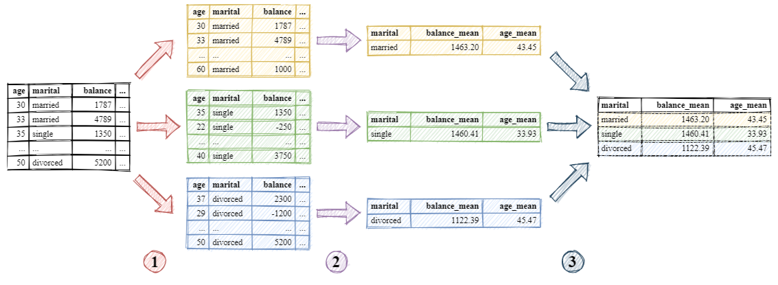
Group By

Group by refers to a 3-step process

1. Splitting the data into groups based on some criteria (e.g., by marital status)
2. Applying a function to each group separately
   • Aggregation (e.g., computing summary statistics)
   • Transformation (e.g., standardization, NA filling, …)
   • Filtering (e.g., remove groups with few rows or based on group aggregates, …)
3. Combining the results into a data structure (a DataFrame most of the time)

(i) If this sounds familiar to you, it is because this is how value_counts() works.

(i) Refer to the documentation for details on DataFrameGroupBy objects and possible aggregations and transformations.

Example: group by marital status and calculate the min, median, and max balance as well as the median age for each group

df.groupby("marital").aggregate(
    # aggregate based on a dict of col_name : 
    # aggregates_list 
    {"balance" : ["min", "median", "max"],
    "age": "median"}
)

	balance			age
	min	median	max	median
marital
married	-3313	452.0	71188	42
single	-1313	462.0	27733	32
divorced	-1148	367.5	26306	45

Example: group by marital status and education level, then calculate median balance, age mean and standard deviation, and number of rows in each group

df.groupby(["marital", "education"]).aggregate(
    # aggregate based on kwarg = (column, aggregate) 
    balance_median = ("balance", "median"),
    age_mean = ("age", "mean"),
    age_std = ("age", "std"),
    count = ("marital", "count")
).reset_index()
# reset idx to more marital & ducation back as cols

	marital	education	balance_median	age_mean	age_std	count
0	married	primary	400.5	47.511407	10.594826	526
1	married	secondary	406.0	42.404345	10.113719	1427
2	married	tertiary	593.0	41.777166	9.574839	727
3	married	unknown	559.0	48.444444	9.587568	117
4	single	primary	538.0	37.013699	9.888957	73
5	single	secondary	376.0	33.052545	7.120707	609
6	single	tertiary	613.5	34.512821	7.217769	468
7	single	unknown	526.5	34.652174	9.175371	46
8	divorced	primary	328.0	51.392405	11.339083	79
9	divorced	secondary	319.5	43.496296	9.333056	270
10	divorced	tertiary	442.0	45.148387	9.340454	155
11	divorced	unknown	774.0	50.375000	10.672242	24

---

Reshaping Dataframes

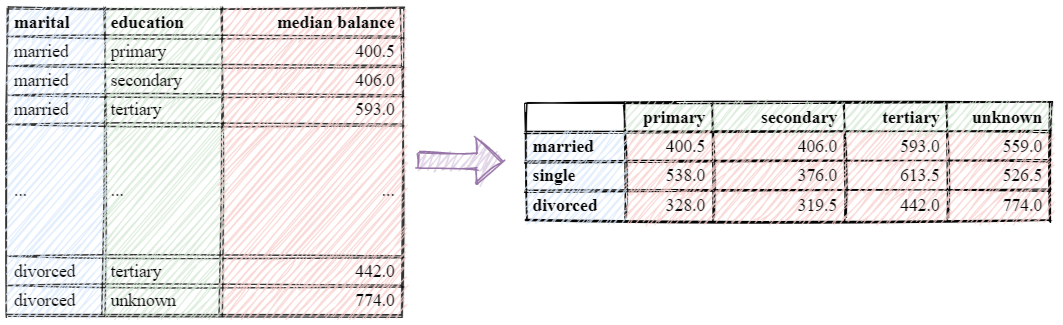
Pivoting

Pivoting is useful when studying how a given (numeric) variable is conditioned by two or more (discrete) variables
- The conditioning variables’ values are used as dimensions (row and column indexes)
- The cells contain the values of the conditioned variable for the corresponding dimensions

df_aggs = df.groupby(["marital", "education"]).aggregate(
    balance_median = ("balance", "median")
).reset_index()
df_aggs

	marital	education	balance_median
0	married	primary	400.5
1	married	secondary	406.0
2	married	tertiary	593.0
3	married	unknown	559.0
4	single	primary	538.0
5	single	secondary	376.0
6	single	tertiary	613.5
7	single	unknown	526.5
8	divorced	primary	328.0
9	divorced	secondary	319.5
10	divorced	tertiary	442.0
11	divorced	unknown	774.0

df_aggs_pivoted = df_aggs.pivot(
    index="marital", columns="education", values="balance_median"
)
df_aggs_pivoted

education	primary	secondary	tertiary	unknown
marital
married	400.5	406.0	593.0	559.0
single	538.0	376.0	613.5	526.5
divorced	328.0	319.5	442.0	774.0

responses_per_marital = df.groupby(["marital", "y"]).aggregate(
    count = ("y", "count")
).reset_index()
responses_per_marital

	marital	y	count
0	married	0	2520
1	married	1	277
2	single	0	1029
3	single	1	167
4	divorced	0	451
5	divorced	1	77

responses_pivoted = responses_per_marital.pivot(index="marital", columns="y", values="count")
responses_pivoted

y	0	1
marital
married	2520	277
single	1029	167
divorced	451	77

response_pct = 100 * responses_pivoted.divide(responses_pivoted.sum(axis="columns"), axis="index")
response_pct

y	0	1
marital
married	90.096532	9.903468
single	86.036789	13.963211
divorced	85.416667	14.583333

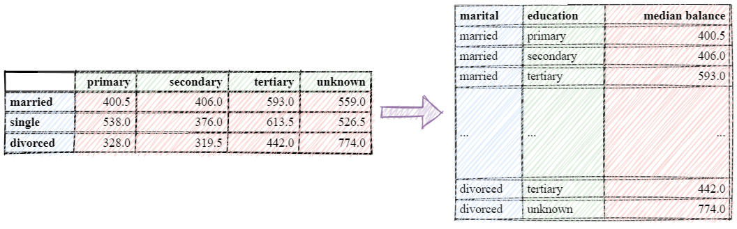
Melting

Melting can be seen as the inverse of pivoting

df_aggs_pivoted

education	primary	secondary	tertiary	unknown
marital
married	400.5	406.0	593.0	559.0
single	538.0	376.0	613.5	526.5
divorced	328.0	319.5	442.0	774.0

df_aggs_pivoted.dtypes

education
primary      float64
secondary    float64
tertiary     float64
unknown      float64
dtype: object

# DOESN'T WORK !!!

#df_aggs_pivoted.reset_index().melt(id_vars="marital", value_name="balance_median")

df_aggs_pivoted.convert_dtypes().reset_index().melt(id_vars="marital", value_name="balance_median")

	marital	variable	balance_median
0	married	primary	400.5
1	single	primary	538.0
2	divorced	primary	328.0
3	married	secondary	406.0
4	single	secondary	376.0
5	divorced	secondary	319.5
6	married	tertiary	593.0
7	single	tertiary	613.5
8	divorced	tertiary	442.0
9	married	unknown	559.0
10	single	unknown	526.5
11	divorced	unknown	774.0

# df_aggs_pivoted.reset_index().melt(id_vars="marital", value_name="balance_median")
# without .convert_dtypes() is doesn't work  
# this could be related to the fact that pandas converts your string columns 
# to categorical columns, which raises an error, if you tries to set a value in a row to 
# a value that is not in the allowed categories (because it was not previously observed).

# A simple fix could be to force all your columns to be string columns instead of pandas-categorical ones, like:

for col in ['Provincia', 'Consumo', 'Potencia max', 'Comercializadora_encoded']:
   df_copy[col] = df_copy[col].astype(str)

Cross Tabulations

Use the crosstab() function to compute cross tabulations (i.e., co-occurrence counts) of two or more categorical Series

• Can be normalized on rows, columns, etc. using the normalize argument
• Can be marginalized by passing margins=True in the function call

# normalize on rows -> yes/no percentage
# in each category of married

# margins=True : sum on columns -> 
# yes/no percentage in all the data frame

100 * pd.crosstab(df["marital"], df["y"],
                 normalize="index",
                 margins=True)

y	no	yes
marital
divorced	85.416667	14.583333
married	90.096532	9.903468
single	86.036789	13.963211
All	88.476001	11.523999

Other Reshaping Operations

Other reshaping operations include

• Stacking and unstacking
• Pivot tables (generalization of the simple pivot)
• Exploding list-like columns
• etc.

---

Working with Multiple Tables

• Real data sets are often organized in multiple data tables
• Each table describes one entity type
  • e.g., a table describes customers, another table describes products, and a third table describes purchases
• Entities can reference other entities they are related to
• In order to conduct your analysis, you need to “patch” these tables together

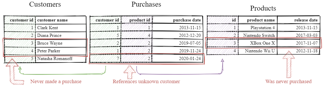
customers = pd.read_csv("retail/customers.csv")
customers.head()

	customer_id	customer_name
0	1	Clark Kent
1	2	Diana Prince
2	3	Bruce Wayne
3	4	Peter Parker
4	5	Natasha Romanoff

purchases = pd.read_csv("retail/purchases.csv")
purchases.head()

	customer_id	product_id	purchase_date
0	1	1	2013-11-15
1	5	4	2012-12-20
2	2	2	2019-07-05
3	1	2	2019-11-24
4	7	2	2020-01-24

products = pd.read_csv("retail/products.csv")
products.head()

	id	product_name	release_date
0	1	PlayStation 4	2013-11-15
1	2	Nintendo Switch	2017-03-03
2	3	XBox One X	2017-11-07
3	4	Nintendo Wii U	2012-11-18

Merging Data Frames

• Use the merge() method to merge a DataFrame with another DataFrame (or Series)
• The merge is done with a database-style (SQL) join
• Usually based on one or more common columns (e.g., the customer_id column in both customers and purchases)
  • If a row from the left object and a row from the right object have matching values for the join columns → a row combining the two is produced
  • If no match is found → output depends on the join type
    • Inner join → no row is produced
    • Left join → for left rows with no match, produce a row (with NA filled right row)
    • Right join → for right rows with no match, produce a row (with NA filled left row)
    • Outer join → combination of left and right join
• Joins can also be performed on rows (less common)

Inner Join

customers.merge(purchases, on="customer_id")

	customer_id	customer_name	product_id	purchase_date
0	1	Clark Kent	1	2013-11-15
1	1	Clark Kent	2	2019-11-24
2	2	Diana Prince	2	2019-07-05
3	5	Natasha Romanoff	4	2012-12-20

Left join

customers.merge(purchases, on="customer_id", how="left")

	customer_id	customer_name	product_id	purchase_date
0	1	Clark Kent	1.0	2013-11-15
1	1	Clark Kent	2.0	2019-11-24
2	2	Diana Prince	2.0	2019-07-05
3	3	Bruce Wayne	NaN	NaN
4	4	Peter Parker	NaN	NaN
5	5	Natasha Romanoff	4.0	2012-12-20

Right join

customers.merge(purchases, on="customer_id", how="right")

	customer_id	customer_name	product_id	purchase_date
0	1	Clark Kent	1	2013-11-15
1	5	Natasha Romanoff	4	2012-12-20
2	2	Diana Prince	2	2019-07-05
3	1	Clark Kent	2	2019-11-24
4	7	NaN	2	2020-01-24

Outer join

customers.merge(purchases, on="customer_id", how="outer")

	customer_id	customer_name	product_id	purchase_date
0	1	Clark Kent	1.0	2013-11-15
1	1	Clark Kent	2.0	2019-11-24
2	2	Diana Prince	2.0	2019-07-05
3	3	Bruce Wayne	NaN	NaN
4	4	Peter Parker	NaN	NaN
5	5	Natasha Romanoff	4.0	2012-12-20
6	7	NaN	2.0	2020-01-24

• Multiple tables can be merged together (consecutively)
• Sometimes, the merge is on columns that do not have the same names (e.g., the id column in products and the product_id column in purchases)
  • Use the left_on and right_on arguments to specify the column names in the left and right data frames respectively

customers.merge(
    # if the merge is on columns that have the
    # same name -> the on arg is optional
    purchases,
).merge(
    products,
    # name of column on left side
    left_on="product_id",
    # name of column on right side
    right_on="id"
).drop("id", axis="columns")
# drop the duplicated column

	customer_id	customer_name	product_id	purchase_date	product_name	release_date
0	1	Clark Kent	1	2013-11-15	PlayStation 4	2013-11-15
1	1	Clark Kent	2	2019-11-24	Nintendo Switch	2017-03-03
2	2	Diana Prince	2	2019-07-05	Nintendo Switch	2017-03-03
3	5	Natasha Romanoff	4	2012-12-20	Nintendo Wii U	2012-11-18

Other tips & tricks

Configure Options & Settings at Interpreter Startup

Highlight all negative values in a dataframe

def color_negative_red(val):
    color = 'red' if val < 0 else 'black'
    return 'color: %s' % color


df = pd.DataFrame(dict(col_1=[1.53,-2.5,3.53], 
                       col_2=[-4.1,5.9,0])
                 )
df.style.applymap(color_negative_red)

	col_1	col_2
0	1.530000	-4.100000
1	-2.500000	5.900000
2	3.530000	0.000000

Pandas options

pd.options.display.max_columns = 50  # None -> No Restrictions  
pd.options.display.max_rows = 200    # None -> Be careful with this   
pd.options.display.max_colwidth = 100  
pd.options.display.precision = 3  

Add row total and column total to a numerical dataframe

df = pd.DataFrame(dict(A=[2,6,3],
                       B=[2,2,6], 
                       C=[3,2,3]))

df['col_total']     = df.apply(lambda x: x.sum(), axis=1)
df.loc['row_total'] = df.apply(lambda x: x.sum())

df

	A	B	C	col_total
0	2	2	3	7
1	6	2	2	10
2	3	6	3	12
row_total	11	10	8	29

Check memory usage

df.memory_usage(deep=True)

Index        170
A             32
B             32
C             32
col_total     32
dtype: int64

Cumulative sum

df = pd.DataFrame(dict(A=[2,6,3],
                       B=[2,2,6], 
                       C=[3,2,3]))

df['cumulative_sum'] = df['A'].cumsum()
df

	A	B	C	cumulative_sum
0	2	2	3	2
1	6	2	2	8
2	3	6	3	11

Crosstab
When you need to count the frequencies for groups formed by 3+ features, pd.crosstab() can make your life easier.

df = pd.DataFrame(dict(
    departure=['SFO', 'SFO', 'LAX', 'LAX', 'JFK', 'SFO'],
    arrival=['ORD', 'DFW', 'DFW', 'ATL', 'ATL', 'ORD'],
    airlines=['Delta', 'JetBlue', 'Delta', 'AA', 'SoutWest', 'Delta']
))

pd.crosstab(
    index=[df['departure'], df['airlines']],
    columns=[df['arrival']],
    rownames=['departure', 'airlines'],
    colnames=['arrival'],
    margins=True # add subtotal
)

	arrival	ATL	DFW	ORD	All
departure	airlines
JFK	SoutWest	1	0	0	1
LAX	AA	1	0	0	1
	Delta	0	1	0	1
SFO	Delta	0	0	2	2
	JetBlue	0	1	0	1
All		2	2	2	6

credits for this tip: Shiu-Tang Li