

Numpy - All You Need To Know
Introduction
I wanted to revise what i’ve learnt so far when dealing with numpy… So i’ve started to create a cheat-sheet. Most of what you’ll find below is taken from Khalil El Mahrsi’s course that you can find on his website smellydatascience.com published under the Creative Commons Attribution-NonCommercial-ShareAlike 4.0 International Public License (CC BY-NC-SA 4.0). So all the credits goes to him. I’ve added few tips found here and there…
I’ve also found a great Visual Intro to NumPy and Data Representation by Jay Alammar that is really interesting ! so let’s begin
Let’s begin :)
What is NumPy?
A fundamental Python package for scientific computation
Which Python data science packages reliy on NumPy?
Many, among others: pandas, scikit-learn, matplotlib…
What do NumPy provide?
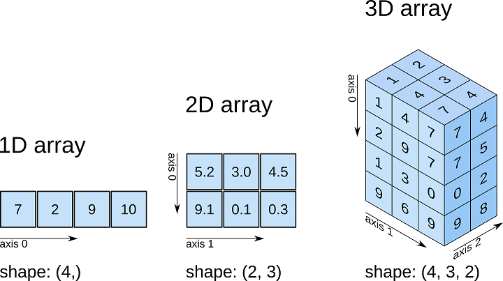
- An object type (the ndarray) for representing multidimensional arrays (vectors, matrices, tensors, …)
- Optimized routines and array operations
- Shape manipulation (indexing and slicing, reshaping, …)
- Linear algebra and mathematical operations
- Statistics
- Random simulation
- Discrete Fourier transforms
Installing & importing Numpy
conda install numpy
pip install numpy
import numpy as np
np.__version__
'1.20.1'
Asking For Help
np.info(np.ndarray.dtype)
Data-type of the array's elements.

Parameters
----------
None

Returns
-------
d : numpy dtype object

See Also
--------
numpy.dtype

Examples
--------
>>> x
array([[0, 1],
       [2, 3]])
>>> x.dtype
dtype('int32')
>>> type(x.dtype)
<type 'numpy.dtype'>
Create an array from a list
a = np.array([10, 9, 8, 7, 6, 5])
a
array([10, 9, 8, 7, 6, 5])
type(a)
numpy.ndarray
np arrays are subscriptable
a[2]
8
slicing is also supported
a[1::2]
array([9, 7, 5])
a[:2]
array([10, 9])
np arrays are mutable
a[3] = 1000
a
array([ 10, 9, 8, 1000, 6, 5])
Why Not Just Use Lists?
Lists are general-purpose sequences.
- Efficient when it comes to insertions, deletions, appending, …
- No support for vectorized operations (e.g., element-wise addition or multiplication)
- Mixed types → must store type info for every item
NumPy arrays are (way) more efficient
- Fixed type (i.e., all elements of an array have the same type)
- Less in-memory space
- No type checking when iterating
- Use contiguous memory → faster access and better caching
- Relies on highly-optimized compiled C code
- Support of vectorization and broadcasting
np.int64
np.float32
np.complex
np.bool
np.object
np.string_
np.unicode_
NumPy Arrays vs. Lists
l1, l2 = [0, 1, 2, 3], [4, 5, 6, 7]
a1, a2 = np.array(l1), np.array(l2)
l1 + l2
[0, 1, 2, 3, 4, 5, 6, 7]
adding two np arrays results in…
elt-wise addition :
a1 + a2
array([ 4, 6, 8, 10])
the * results in list replication
…but results in elt-wise multiplication for ndarrays
3 * l1
[0, 1, 2, 3, 0, 1, 2, 3, 0, 1, 2, 3]
3 * a1
array([0, 3, 6, 9])
trying to multiply lists raises an exception…
…but is supported for ndarrays
l1 * l2
---------------------------------------------------------------------------

TypeError                                 Traceback (most recent call last)

<ipython-input-17-ec7519df584c> in <module>
----> 1 l1 * l2


TypeError: can't multiply sequence by non-int of type 'list'
a1 * a2
array([ 0, 5, 12, 21])
What make NumPy significantly faster than built-in Python lists?
Vectorization, fixed types, compiled C implementations, etc…
l = list(range(10000))
a = np.array(l)
%%timeit -n 10000 -r 10
sum([2 * i for i in l])
975 µs ± 28.6 µs per loop (mean ± std. dev. of 10 runs, 10000 loops each)
%%timeit -n 10000 -r 10
(2 * a).sum()
21.1 µs ± 1.26 µs per loop (mean ± std. dev. of 10 runs, 10000 loops each)
NumPy Array Basics
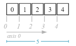
Attributes of interest:
- shape
- ndim
- dtype
- itemsize
- nbytes
number of dimensions
a = np.array([0, 1, 2, 3, 4])
a.ndim
1
shape (length along each dimension)
a.shape
(5,)
data type
a.dtype
dtype('int32')
itmen size in bytes
a.itemsize
4
total memory size in bytes
a.nbytes
20
positional indexing works the same as lists
a[1]
1
same goes for slicing
a[1:4]
array([1, 2, 3])
arrays are mutable but beware of type coercion!
a[4] = 12.5
a
array([ 0, 1, 2, 3, 12])
Multi-Dimensional Arrays
For the sake of simplification, examples shown here use two-dimensional arrays. The principles remains the same for arrays of higher dimensions.
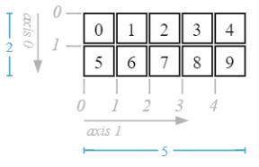
b = np.array([
    [0, 1, 2, 3, 4],  # 1st row
    [0, 1, 2, 3, 4]], # 2nd row
    # type eventually specified
    dtype=np.int16)

b.ndim
2
b.shape
(2, 5)
b.dtype
dtype('int16')
b.itemsize
2
b.nbytes
20
For 3D arrays:
Basic Array Indexing
NumPy’s basic array indexing and slicing are extensions of Python’s indexing and slicing to N dimensions
- One slice or index per dimension
- Separated by a comma (,)
Similar rules apply to omitted parts of a slice
- d_i_start omitted → 0
- d_i_end omitted → array.shape[i]
- d_i_step omitted → 1
If a dimension is to be fully retained, use a colon (:) as the corresponding slice
Syntax (indexing)
array[i, j, …]
Syntax (slicing)
array[d_0_start: d_0_end: d_1_step, d_1_start: d_1_end: d_1_step, …]
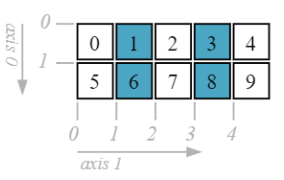
Basic Array Indexing
Access a single item
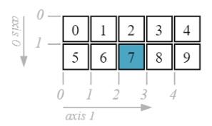
d = np.array([
[0, 1, 2, 3, 4],
[5, 6, 7, 8, 9]])
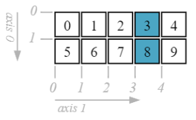
d[1, 2]
7
Access a whole row
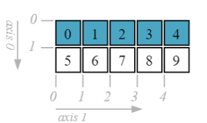
d[0, :] # d[0]
array([0, 1, 2, 3, 4])
Asscess a whole column
d[:, 3]
array([3, 8])
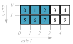
d[:, :3]
array([[0, 1, 2],
       [5, 6, 7]])
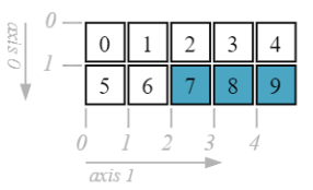
d[1, 2:]
array([7, 8, 9])
d[:, 1::2]
array([[1, 3],
       [6, 8]])
d[:, [1, 3]]
array([[1, 3],
       [6, 8]])
Array Content Modification
- NumPy arrays are mutable
- Indexing and slicing can be used in assignment statements to modify items
- Values are coerced to the array’s data type (e.g., the decimal part of a float will be truncated when it is inserted in an array of integers)
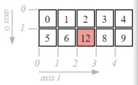
e = np.array([
    [0, 1, 2, 3, 4],
    [5, 6, 7, 8, 9]])

e[1, 2] = 12.9
e
array([[ 0,  1,  2,  3,  4],
       [ 5,  6, 12,  8,  9]])
Modify multiple items through slicing
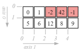
d[0, 2:] = [-2, 42, -1]
d
array([[ 0,  1, -2, 42, -1],
       [ 5,  6,  7,  8,  9]])
Modify multiple items through slicing (with broadcasting)
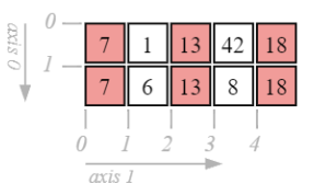
d[:, ::2] = [7, 13, 18]
d
array([[ 7,  1, 13, 42, 18],
       [ 7,  6, 13,  8, 18]])
Modify multiple items through boolean filtering (will be presented later)
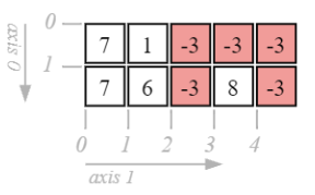
d[d >= 13] = -3
d
array([[ 7,  1, -3, -3, -3],
       [ 7,  6, -3,  8, -3]])
Returns copy with values appended. NOT in-place
x = np.array([0,1,2,3,4])
y = np.append(x, [5,6,7,8,9])
x
array([0, 1, 2, 3, 4])
y
array([0, 1, 2, 3, 4, 5, 6, 7, 8, 9])
When dealing with arrays with higher dimensions, we use : for selecting the whole indices along each axis. We can also use … can select all indices across multiple axes. The exact number of axes expanded is inferred.
arr = np.array(range(30)).reshape(2, 5, -1)
arr
array([[[ 0,  1,  2],
        [ 3,  4,  5],
        [ 6,  7,  8],
        [ 9, 10, 11],
        [12, 13, 14]],

       [[15, 16, 17],
        [18, 19, 20],
        [21, 22, 23],
        [24, 25, 26],
        [27, 28, 29]]])
c[1, ...] #Same as [1, :, :]
arr[..., 2]
array([[ 2,  5,  8, 11, 14],
       [17, 20, 23, 26, 29]])
Insert an item in an array
a = np.arange(5)
np.insert(a, 1, 100)
array([ 0, 100, 1, 2, 3, 4])
Delete an item in an array
a = np.arange(5)[: :-1]
np.delete(a, 2)
array([4, 3, 1, 0])
Arithmetic Operations and Basic Math
- NumPy arrays support a wide range of element-wise arithmetic operations (sum, substraction, multiplication, …)
- NumPy also provides a wide range of mathematical functions
- Trigonometric and hyperbolic functions
- Sums, products, and differences over axes
- Logarithms and exponents
- …
Most array operations can be vectorized. Do not use for loops unless it is absolutely necessary (very rare)!
element-wise sum of 2 arrays
a = np.array([0, 1, 2])
b = np.array([3, 4, 5])
a + b
array([3, 5, 7])
element-wise product
a = np.array([0, 1, 2])
b = np.array([3, 4, 5])
a * b * b
array([ 0, 16, 50])
element-wise power
a = np.array([0, 1, 2])
b = np.array([3, 4, 5])
a ** b
array([ 0, 1, 32], dtype=int32)
trigonometric functions (sin, cos, tan)
a = np.array([0, 1, 3.14/2])
np.sin(a)
array([0. , 0.84147098, 0.99999968])
hyperbolic functions (sinh, cosh, tanh)
a = np.array([0, 1, 3.14/2])
np.tanh(a)
array([0. , 0.76159416, 0.91702576])
log and exponential functions
a = np.array([1, 10, 100])
np.log(a)
array([0. , 2.30258509, 4.60517019])
sum all the matrix’s elements
m = np.array([
    [0, 1, 2, 3, 4],
    [5, 6, 7, 8, 9]])

np.sum(m)
45
sum along the rows
m = np.array([
    [0, 1, 2, 3, 4],
    [5, 6, 7, 8, 9]])

np.sum(m, axis = 0)
array([ 5, 7, 9, 11, 13])
sum along the columns
m = np.array([
    [0, 1, 2, 3, 4],
    [5, 6, 7, 8, 9]])

np.sum(m, axis = 1)
array([10, 35])
difference along the columns
m = np.array([
    [0, 1, 2, 3, 4],
    [5, 6, 7, 8, 9]])

np.diff(m, axis=1)
array([[1, 1, 1, 1],
       [1, 1, 1, 1]])
product along the rows
m = np.array([
    [0, 1, 2, 3, 4],
    [5, 6, 7, 8, 9]])

np.prod(m, axis=0)
array([ 0, 6, 14, 24, 36])
Element-wise comparison between 2 arrays
a = np.array([1, 2, 3])
b = np.array([0, 2, 0])
a == b
array([False, True, False])
Array-wise comparison
np.array_equal(a, b)
False
Element-wise comparison
a = np.array([1, 2, 3])
a < 2
array([ True, False, False])
Broadcasting
- Broadcasting designates how NumPy conducts arithmetic operations on arrays with different shapes
- If the arrays have compatible dimensions
- The smaller array is “replicated” to match the bigger array’s dimensions
- The operation is conducted element-wise as usual
- If the arrays have incompatible dimensions, a ValueError is raised
- Dimensions are compatible if
- They are equal, or
- One of them is 1
Broadcasting a scalar
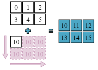
a = np.array([[0, 1, 2],
             [3, 4, 5]])
a + 10
array([[10, 11, 12],
       [13, 14, 15]])
Broadcasting a row
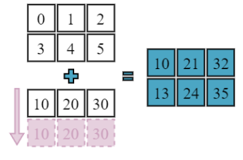
a = np.array([[0, 1, 2],
             [3, 4, 5]])
b = np.array([10, 20, 30])
a + b
array([[10, 21, 32],
       [13, 24, 35]])
Broadcasting a colum
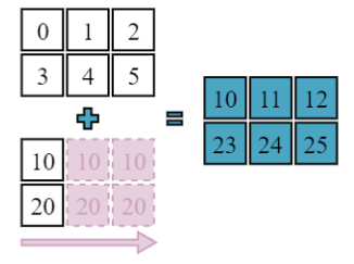
a = np.array([[0, 1, 2],
             [3, 4, 5]])
b = np.array([[10], [100]])
a + b
array([[ 10,  11,  12],
       [103, 104, 105]])
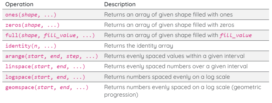
Array Creation Routines
NumPy provides useful routines for creating arrays (filled with constant values, from numeric ranges, …)
np.zeros((3, 4))
array([[0., 0., 0., 0.],
       [0., 0., 0., 0.],
       [0., 0., 0., 0.]])
np.ones((3, 2), dtype=np.int32)
array([[1, 1],
       [1, 1],
       [1, 1]])
np.full([2, 3], 42)
array([[42, 42, 42],
       [42, 42, 42]])
a = np.array([[0, 1], [3, 4]])
np.full_like(a, 66, dtype=np.float16)
array([[66., 66.],
       [66., 66.]], dtype=float16)
# same as np.eye(4)
np.identity(4)
array([[1., 0., 0., 0.],
       [0., 1., 0., 0.],
       [0., 0., 1., 0.],
       [0., 0., 0., 1.]])
Create an empty array
np.empty((3,2))
array([[0., 0.],
       [0., 0.],
       [0., 0.]])
np.diag(np.arange(4))
array([[0, 0, 0, 0],
       [0, 1, 0, 0],
       [0, 0, 2, 0],
       [0, 0, 0, 3]])
creates an array from start to stop in step.
np.arange(start, stop, step)
np.arange(0, 1.1, 0.25)
array([0. , 0.25, 0.5 , 0.75, 1. ])
given an array containing some numbers and a range, limit the numbers to that range.
For numbers outside the range, it returns the edge value.
a = np.arange(10)
np.clip(a, 3, 5)
array([3, 3, 3, 3, 4, 5, 5, 5, 5, 5])
return an array with the evenly spaced numbers from strat to stop
np.linespace(start, stop, num)
np.linspace(0, 20, 5)
array([ 0., 5., 10., 15., 20.])
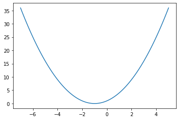
It is convenient to draw math function:
import matplotlib.pyplot as plt

def f(x): return x**2 + 2*x + 1

x = np.linspace(-7, 5, 100)
plt.plot(x, f(x))
plt.show()
np.logspace(1, 5, num=3)
array([1.e+01, 1.e+03, 1.e+05])
np.geomspace(1, 1000, 4)
array([ 1., 10., 100., 1000.])
Random Number Generation Routines
NumPy provides useful random number generation and sampling routines
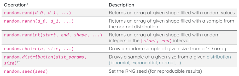 *These are the legacy operations that you will see the most in code examples. NumPy also provides updated routines (recommended)
** distribution is to be replaced by the distribution’s name
generates random numbers uniformly distributed between 0 to 1 in a given shape.
rand()
np.random.rand(5)
array([0.28977318, 0.36827695, 0.43480548, 0.62994031, 0.90077232])
# fix seed
np.random.seed(42)
np.random.rand(3, 2)
array([[0.37454012, 0.95071431],
       [0.73199394, 0.59865848],
       [0.15601864, 0.15599452]])
generates an array (size=size) of random integers in the range (low — high).
randint(low, high, size)
np.random.seed(42)
np.random.randint(20, 100, size=5)
array([71, 34, 91, 80, 40])
randomly choose samples from a given array. It is also possible to pass a probability.
random.choice()
x = [0, 1, 2, 3, 4, 5]
np.random.choice(x, 10)
array([0, 0, 0, 4, 2, 1, 4, 3, 1, 3])
a = np.arange(10)
np.random.seed(42)

# default w/replacement
np.random.choice(a, size=5)
array([6, 3, 7, 4, 6])
np.random.seed(42)
np.random.binomial(n=1, p=0.5, size=10)
array([0, 1, 1, 1, 0, 0, 0, 1, 1, 1])
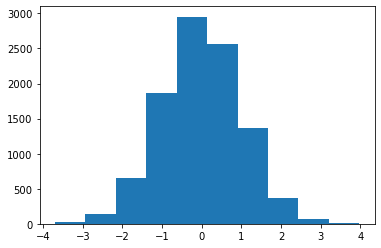
generates random numbers in a normal distribution.
randn()
plt.hist(np.random.randn(10000))
plt.show()
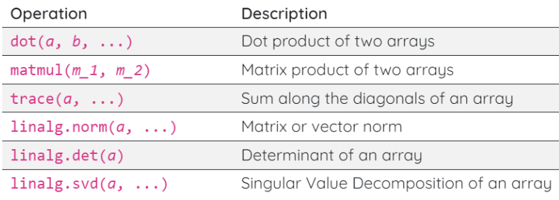
Linear Algebra
NumPy provides optimized implementations of linear algebra functions
a = np.array([0, 1, 2])
b = np.array([3, 4, 5])
np.dot(a, b)
# equivalent to np.sum(a * b)
14
dot product (or more generally matrix multiplication) is done with a function
a = np.array([[0, 1, 2], [3, 4, 5]])
b = np.array([[0, 1], [1, 1], [1, 0]])
np.dot(a, b)
array([[3, 1],
       [9, 7]])
In Python 3.5, the @ operator was added as an infix operator for matrix multiplication
x = np.diag(np.arange(4))
x@x
array([[0, 0, 0, 0],
       [0, 1, 0, 0],
       [0, 0, 4, 0],
       [0, 0, 0, 9]])
a = np.array([[0, 1, 2],
              [3, 4, 5],
              [7, 8, 9]])

np.trace(a)
13
a = np.array([1, 2, 3])
# equivalent: np.sqrt(np.dot(a, a))
np.linalg.norm(a)
3.7416573867739413
a = np.array([[1, 2, 3],
              [4, 5, 6],
              [7, 8, 9]])

# matrix's Frobenius norm
np.linalg.norm(a)
16.881943016134134
a = np.array([[1, 2, 3],
              [4, 5, 6],
              [7, 8, 9]])

# matrix's Frobenius norm
np.linalg.matrix_power(a, 3)
array([[ 468,  576,  684],
       [1062, 1305, 1548],
       [1656, 2034, 2412]])
a = np.arange(9).reshape(3, -1)
# same as a.T
np.transpose(a)
array([[0, 3, 6],
       [1, 4, 7],
       [2, 5, 8]])
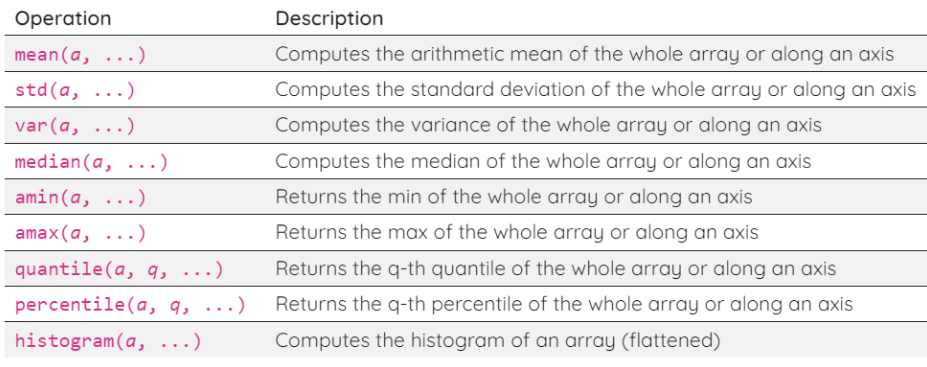
Statistics
NumPy provides multiple routines for statistics
a = np.array([[1, 4, -3],
              [0, 7, 2],
              [9, 3, 4]])

np.mean(a)
3.0
a = np.array([[1, 4],
              [0, 7],
              [9, 3]])

np.mean(a, axis=1)
array([2.5, 3.5, 6. ])
a = np.array([[1, 4, -3],
              [0, 7, 2],
              [9, 3, 4]])

np.median(a, axis=1)
array([1., 2., 4.])
a = np.array([[1, 4, -3],
              [0, 7, 2],
              [9, 3, 4]])

# np.max(a, axis=0) also works
np.amax(a, axis=0)
array([9, 7, 4])
a = np.array([[1, 4, -3],
              [0, 7, 2],
              [9, 3, 4]])

np.min(a, axis=1)
array([-3, 0, 3])
returns the indices of the max values along an axis.
useful in object classification and detection to find the object with the highest probability.
There are also similar functions like argmin() , argwhere() , argpartition()
a = np.array([[1, 4, -3],
              [0, 7, 2],
              [9, 3, 4]])

# index of min along each col
np.argmin(a, axis=1)
array([2, 0, 1], dtype=int64)
For an array arr, np.argmax(arr), np.argmin(arr), and np.argwhere(condition(arr)) return the indices of maximum values, minimum values, and values that satisfy a user-defined condition respectively. While these arg functions are widely used, we often overlook the function np.argsort() that returns the indices that would sort an array.
We can use np.argsort to sort values of arrays according to another array. Here is an example of sorting student names using their exam scores. The sorted name array can also be transformed back to its original order using np.argsort(np.argsort(score)).
score = np.array([70, 60, 50, 10, 90, 40, 80])
name = np.array(['Ada', 'Ben', 'Charlie', 'Danny', 'Eden', 'Fanny', 'George'])

# # an array of names in ascending order of their scores
sorted_names = name[np.argsort(score)]
sorted_names
array(['Danny', 'Fanny', 'Charlie', 'Ben', 'Ada', 'George', 'Eden'],
      dtype='<U7')
sorted_names[np.argsort(np.argsort(score))]
array(['Ada', 'Ben', 'Charlie', 'Danny', 'Eden', 'Fanny', 'George'],
      dtype='<U7')
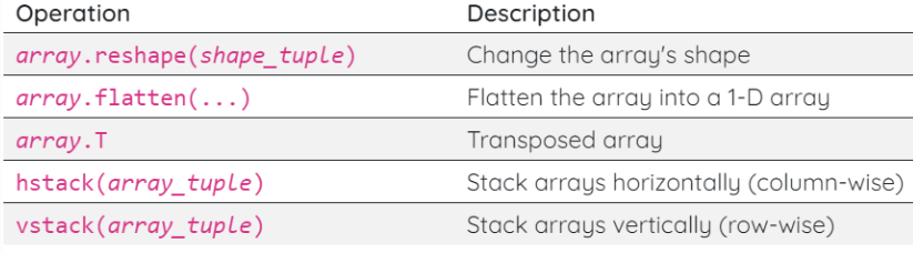
Reshaping Arrays
Array manipulation routines can be used to change array shapes, join arrays, …
reshape a multidimensional array to 1D array
flatten a into a 1-D array
a = np.array([[0, 1, 2], [3, 4, 5]])
a
array([[0, 1, 2],
       [3, 4, 5]])
a.flatten()
array([0, 1, 2, 3, 4, 5])
a = np.array([[0, 1, 2], [3, 4, 5]])
a
array([[0, 1, 2],
       [3, 4, 5]])
reshape the array
a = np.array([[0, 1, 2], [3, 4, 5]])

a.reshape(3, 2)
array([[0, 1],
       [2, 3],
       [4, 5]])
we can use -1 , numpy calculates the dimension for you.
a = np.array([0, 1, 2, 3, 4, 5])

a.reshape((2, -1))
array([[0, 1, 2],
       [3, 4, 5]])
stack arrays horizontally
(arrays are provided as tuples)
a = np.array([[0, 1, 2], [3, 4, 5]])
b = np.array([[0, 10, 20], [30, 40, 50]])
np.hstack((a, b))
array([[ 0,  1,  2,  0, 10, 20],
       [ 3,  4,  5, 30, 40, 50]])
stack arrays horizontally
(arrays are provided as tuples)
a = np.array([[0, 1, 2], [3, 4, 5]])
b = np.array([[0, 10, 20], [30, 40, 50]])
c = np.vstack((a, b))
c
array([[ 0,  1,  2],
       [ 3,  4,  5],
       [ 0, 10, 20],
       [30, 40, 50]])
split array vertically into 4 arrays
a = np.array([[0, 1, 2], [3, 4, 5]])
b = np.array([[0, 10, 20], [30, 40, 50]])
c = np.vstack((a, b))

np.vsplit(c, 4)
[array([[0, 1, 2]]),
 array([[3, 4, 5]]),
 array([[ 0, 10, 20]]),
 array([[30, 40, 50]])]
how to insert a new axis at a user-defined axis position ?
with np.newaxis, this operation expands the shape of an array by one unit of dimension. While this can also be done by np.expand_dims(), using np.newaxis is much more readable and arguably more elegant
arr = np.array(range(1000)).reshape(2,5,4,-1)
arr.shape
(2, 5, 4, 25)
arr[..., np.newaxis, :, :, :].shape
(2, 1, 5, 4, 25)
Remove single-dimensional entries from the shape of an array
x = np.array([[[0], [1], [2]]])
x
array([[[0],
        [1],
        [2]]])
np.squeeze(x)
array([0, 1, 2])
np.squeeze(x, axis=0)
array([[0],
       [1],
       [2]])
Advanced Indexing
In addition to standard (basic) Python indexing, NumPy supports a more advanced indexing syntax
- Using integer array indexing
- With boolean “masking”
an example of advanced integer array indexing
a = np.array([
    [-2, 50, 23, 30],
    [42, -7, -8, 11],
    [40, 20, 15, 17]
])

a[[0, 2, 1], [2, 1, 1]]
array([23, 20, -7])
positions to retain on each row using the a boolean ndarray to mask / filter values
a = np.array([
    [-2, 50, 23, 30],
    [42, -7, -8, 11],
    [40, 20, 15, 17]
])

filter = np.array([
    [False, False, False, True ],
    [True,  True,  True,  False],
    [False, True,  False, True ]
])

a [filter]
array([30, 42, -7, -8, 20, 17])
conducts elt-wise truth value testing -> result used as filter
a = np.array([
    [-2, 50, 23, 30],
    [42, -7, -8, 11],
    [40, 20, 15, 17]
])

a[a < 0]
array([-2, -7, -8])
| boolean ndarrays can be combined with & (and) and | (or) |
a = np.array([
    [-2, 50, 23, 30],
    [42, -7, -8, 11],
    [40, 20, 15, 17]
])

a[(a > 10) & (a < 40)]
array([23, 30, 11, 20, 15, 17])
a[(a < 0) | (a > 40)]
array([-2, 50, 42, -7, -8])
advanced indexes can be used to modify elts
a = np.array([
    [-2, 50, 23, 30],
    [42, -7, -8, 11],
    [40, 20, 15, 17]
])

a[(a < 0) | (a > 40)] = 99
a
array([[99, 99, 23, 30],
       [99, 99, 99, 11],
       [40, 20, 15, 17]])
Numpy has a submodule numpy.ma that supports data arrays with masks. A masked array contains an ordinary numpy array and a mask that indicates the position of invalid entries.
np.ma.MaskedArray(data=arr, mask=invalid_mask)
import numpy.ma as ma
x = np.array([1, 2, 3, -1, 5])

mx = ma.masked_array(x, mask=[0, 0, 0, 1, 0])
mx
masked_array(data=[1, 2, 3, --, 5],
             mask=[False, False, False,  True, False],
       fill_value=999999)
Other tips and tricks
returns the values in an array that are not in another array.
a = np.array([1, 2, 3, 4, 5, 6])
b = np.array([4, 5, 6, 7, 8, 9])
np.setdiff1d(a, b)
array([1, 2, 3])
np.setdiff1d(b, a)
array([7, 8, 9])
returns the intersection of 2 arrays
a = np.array([1, 2, 3, 4, 5, 6])
b = np.array([4, 5, 6, 7, 8, 9])
np.intersect1d(a, b)
array([4, 5, 6])
returns elements chosen from x or y depending on condition.
exam_scores = np.array([40, 80, 90, 20])
np.where(exam_scores > 60, 'pass', 'fail')
array(['fail', 'pass', 'pass', 'fail'], dtype='<U4')
If the x and y are not passed to the np.where , the index position of the elements that meet the condition will be returned.
np.where(exam_scores > 60)
(array([1, 2], dtype=int64),)
how to sort an array
a = np.array([3, 2, 1])
a.sort()
a
array([1, 2, 3])
a = np.array([
    [9, 8, 6],
    [3, 2, 1]
])
a.sort(axis=0)
a
array([[3, 2, 1],
       [9, 8, 6]])
Reverse an array
a = np.arange(10)
a[ : :-1]
array([9, 8, 7, 6, 5, 4, 3, 2, 1, 0])
Copying Arrays
Create a view of the array with the same data
h = a.view()
Create a copy of the array
np.copy(a)
Create a deep copy of the array
h = a.copy()
