

Cirta - Particle Type Classification - Part 2/2
Banner made from a photo by Max Bender on Unsplash
This is the second and final part of this challenge. In the first part we’ve prepared the data set and explored it. The goal is to build a machine learning model to help physicists identify particles in images.
Short Introduction
If you’re in a hurry…
Proposed by Zindi
In this challenge we want to build a machine learning model to help us recognize particles. Particles are the tiny constituant of matter generated in a collision between proton bunches at the Large Hadron Collider at CERN.
Particles are of course of different types and identifying which particle was produced in an extremly important task for particle physicists.
Our dataset comprises 350 independent simulated events, where each event contains labelled images of particle trajectories.
A good model assigns the correct particle type to any particle, even the least frequent ones.
Read throught this notebook to discover more about the particles.
Data Preparation
This is the same process as previously done in the 1st part. Let’s create a dictionnary to convert the class numbers to their real names and see how many elements each class is made of.
# code to particle name dictionary :
dic_types = {11: "electron", 13: "muon", 211: "pion", 321: "kaon", 2212: "proton"}
dic_tf = {11: 0, 13: 1, 211: 2, 321: 3, 2212: 4}
y = np.array(pd.DataFrame(y).replace(dic_tf))
np.unique(y, return_counts=True)
(array([0, 1, 2, 3, 4]), array([ 3150, 700, 981050, 160300, 114100]))
As usual, we have to split or data, so that we can train our model and later test it on two different sets :
from sklearn.model_selection import train_test_split

# preprocess dataset, split into training and test part
X_train, X_test, y_train, y_test = train_test_split(X, y, test_size=0.20, random_state=42, stratify=y)
X_train.shape, X_test.shape, y_train.shape, y_test.shape
((1007440, 100), (251860, 100), (1007440, 1), (251860, 1))
nb_classes = len(np.unique(y))
nb_classes
5
With a Deep Learning model made with Tensorflow
Since the images are only composed of a few pixels, there is no need to use a C.N.N model. In this case, a M.L.P (Multi Layer Perceptron) will do the job. At first, it is important to convert the target into categorical features.
from tensorflow.keras.utils import to_categorical

y_train_cat = to_categorical(y_train, num_classes=nb_classes, dtype='int32')
y_test_cat = to_categorical(y_test, num_classes=nb_classes, dtype='int32')
y_train_cat.shape, y_test_cat.shape
((1007440, 5), (251860, 5))
Let’s have a look of our target transformed :
y_train_cat
array([[0, 0, 1, 0, 0],
       [0, 0, 1, 0, 0],
       [0, 0, 1, 0, 0],
       ...,
       [0, 0, 1, 0, 0],
       [0, 0, 0, 0, 1],
       [0, 0, 1, 0, 0]], dtype=int32)
The range of the values of our features spans from 0 to 8 :
X.max(), X.min()
(8.0, 0.0)
The Neural Network in our case uses gradient descent as an optimization algorithm to find the appropriate weights(w) for each feature.
We are using the gradient descent algorithm to optimize the cost function and update the weights. So if some of the features have a very large scale then gradient descent takes more numbers of iterations for that feature to converge as compared to the other features having a small scale and if the feature which has high scale is highly correlated to the target output then the performance of the model will be affected as a whole because the weights for this particular feature will not converge to give the best performance.
#from sklearn.preprocessing import StandardScaler

#scaler = StandardScaler()
#X_train = scaler.fit_transform(X_train)
#X_test = scaler.transform(X_test)

X_train, X_test = X_train / 8, X_test / 8
Base line / first attempt
freq_array = np.unique(y, return_counts=True)
class_weight = {k: d for k, d in zip(freq_array[0], freq_array[1])}
class_weight
{0: 3150, 1: 700, 2: 981050, 3: 160300, 4: 114100}
from sklearn.utils import class_weight

class_weights = class_weight.compute_class_weight('balanced', np.unique(y), y.flatten())
class_weights
array([7.99555556e+01, 3.59800000e+02, 2.56724938e-01, 1.57117904e+00,
       2.20736196e+00])
initial_bias = np.log([700/981050])
initial_bias
array([-7.24529837])
from tensorflow.keras.models import Sequential
from tensorflow.keras.layers import Dense


input_dim = X_train.shape[1]

model = Sequential()
model.add(Dense(20, input_dim=input_dim, activation='relu'))#, use_bias = True, bias_initializer='zeros'))
model.add(Dense(10, activation='relu'))
model.add(Dense(nb_classes, activation='softmax'))


model.compile(loss='sparse_categorical_crossentropy',
              optimizer='SGD', # nadam
              metrics=['accuracy'])
model.summary()
_________________________________________________________________
Layer (type)                 Output Shape              Param #
=================================================================
dense_15 (Dense)             (None, 20)                2020
_________________________________________________________________
dense_16 (Dense)             (None, 10)                210
_________________________________________________________________
dense_17 (Dense)             (None, 5)                 55
=================================================================
Total params: 2,285
Trainable params: 2,285
Non-trainable params: 0
_________________________________________________________________
#model.get_weights()
y_train_cat.shape
(1007440, 5)
model.fit(X_train, y_train,
          class_weight=class_weight,
          epochs=8,
          batch_size=1000,
          validation_data=(X_test, y_test))
Train on 1007440 samples, validate on 251860 samples
Epoch 1/8
1007440/1007440 [==============================] - 2s 2us/sample - loss: 0.6918 - acc: 0.7790 - val_loss: 0.6917 - val_acc: 0.7790
Epoch 2/8
1007440/1007440 [==============================] - 2s 2us/sample - loss: 0.6916 - acc: 0.7790 - val_loss: 0.6916 - val_acc: 0.7790
Epoch 3/8
1007440/1007440 [==============================] - 2s 2us/sample - loss: 0.6915 - acc: 0.7790 - val_loss: 0.6915 - val_acc: 0.7790
Epoch 4/8
1007440/1007440 [==============================] - 2s 2us/sample - loss: 0.6914 - acc: 0.7790 - val_loss: 0.6913 - val_acc: 0.7790
Epoch 5/8
1007440/1007440 [==============================] - 2s 2us/sample - loss: 0.6913 - acc: 0.7790 - val_loss: 0.6912 - val_acc: 0.7790
Epoch 6/8
1007440/1007440 [==============================] - 2s 2us/sample - loss: 0.6912 - acc: 0.7790 - val_loss: 0.6911 - val_acc: 0.7790
Epoch 7/8
1007440/1007440 [==============================] - 2s 2us/sample - loss: 0.6911 - acc: 0.7790 - val_loss: 0.6910 - val_acc: 0.7790
Epoch 8/8
1007440/1007440 [==============================] - 2s 2us/sample - loss: 0.6909 - acc: 0.7790 - val_loss: 0.6909 - val_acc: 0.7790
y_pred_train = model.predict(X_train, batch_size=1000)
from sklearn.metrics import confusion_matrix

confusion_matrix(y_train.flatten(), np.argmax(y_pred_train, axis=1))
array([[     0,      0,   2520,      0,      0],
       [     0,      0,    560,      0,      0],
       [     0,      0, 784840,      0,      0],
       [     0,      0, 128240,      0,      0],
       [     0,      0,  91280,      0,      0]])
from sklearn.metrics import confusion_matrix, log_loss


import itertools
class_names = ['11', '13', '211', '321', '2212']


def plot_confusion_mtx(trained_model):
    """Plot the confusion matrix with color and labels"""
    matrix = confusion_matrix(y_test.flatten(),
                              np.argmax(trained_model.predict(X_test, batch_size=50000),
                              axis=1))
    plt.clf()

    # place labels at the top
    plt.gca().xaxis.tick_top()
    plt.gca().xaxis.set_label_position('top')

    # plot the matrix per se
    plt.imshow(matrix, interpolation='nearest', cmap=plt.cm.Blues)

    # plot colorbar to the right
    plt.colorbar()
    fmt = 'd'

    # write the number of predictions in each bucket
    thresh = matrix.max() / 2.
    for i, j in itertools.product(range(matrix.shape[0]), range(matrix.shape[1])):

        # if background is dark, use a white number, and vice-versa
        plt.text(j, i, format(matrix[i, j], fmt),
             horizontalalignment="center",
             color="white" if matrix[i, j] > thresh else "black")

    tick_marks = np.arange(len(class_names))
    plt.xticks(tick_marks, class_names, rotation=45)
    plt.yticks(tick_marks, class_names)
    plt.tight_layout()
    plt.ylabel('True label',size=14)
    plt.xlabel('Predicted label',size=14)
    plt.show()


def display_confusion_matx(best_model_path):
    if os.path.isfile(best_model_path):
        with open(best_model_path, 'rb') as f:
            best_clf = pickle.load(f)
        plot_confusion_mtx(best_clf)


#display_confusion_matx('1_original_data_LGBMClassifier')
np.unique(y_pred, return_counts=True)
(array([0, 2]), array([3, 3]))
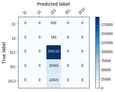
plot_confusion_mtx(model)
2nd try : Using a different model, and changing the parameters
model = Sequential()
input_dim = X_train.shape[1]
nb_classes = y_train.shape[1]

model.add(Dense(10, input_dim=input_dim, activation='relu', name='input'))
model.add(Dense(20, activation='relu', name='fc1'))
model.add(Dense(10, activation='relu', name='fc2'))
model.add(Dense(nb_classes, activation='softmax', name='output'))

model.compile(loss='categorical_crossentropy',
              optimizer='nadam',
              metrics=['accuracy'])


# from sklearn.utils import class_weight
# class_weight = class_weight.compute_class_weight('balanced', np.unique(y_train), y_train)
#class_weight = {0 : 1., 1: 20.}
model.fit(X_train, y_train, epochs=3, batch_size=50000, class_weight={0: 3150, 1: 700, 2: 981050, 3: 160300, 4: 114100})
WARNING:tensorflow:From C:\Anaconda3\lib\site-packages\tensorflow\python\ops\math_ops.py:3066: to_int32 (from tensorflow.python.ops.math_ops) is deprecated and will be removed in a future version.
Instructions for updating:
Use tf.cast instead.
Epoch 1/3
1007440/1007440 [==============================] - 3s 3us/sample - loss: 1.5577 - acc: 0.4882
Epoch 2/3
1007440/1007440 [==============================] - 3s 3us/sample - loss: 1.1783 - acc: 0.7790
Epoch 3/3
1007440/1007440 [==============================] - 3s 3us/sample - loss: 0.5487 - acc: 0.7790
score = model.evaluate(X_test, y_test, batch_size=50000)
score
251860/251860 [==============================] - 0s 1us/sample - loss: 1.0910 - acc: 0.7790

[1.0910033097309182, 0.7790439]
Unfortunately, the results were the same. The predictions weren’t improved ! I’ve not spent many times on this challenge, & should have clearly try other methods. For a moment, i was thinking of stacking various model, probably different models will behave differently depending on the target class, using a stack to get the best of each model could have been a good solution… Now let’s understand the best solution for this challenge proposed by an other Data Scientist !
Best solution by M.S Jedidi
All the credits goes to Mohamed Salam JEDIDI. The original solution can be found on his dedicated github repository. It consitsts in an ensemble of fine-tuned Catboost Classifiers, each one trained on a different portion of the data for some classes (the majority ones). This is a really brillant approach i wasn’t aware of !
Approach : The main problem in this challenge was the class imbalance. You can quickly notice that there are 3 dominant classes with tens of thousands of samples, while 2 classes were having over 1300 samples and the other one around 3k samples. It is also mentioned that the test set was made to be balanced. If you train a model with the data as it is, your model will be predicting the majority classes only due to the severe class imbalance.
Data Preprocessing : the images’ pixels were flattened and stacked in a dataframe, and each column represented a single pixel, and each row represented an image. We then were able to use sklearn and boosting algorithms on the newly created tabular data to perform classification.
1st approach : Oversampling
The oversampling approach didn’t yield good results since there were not too many samples in the minority classes to be able to match the number of samples in the majority classes.
2nd approach : Undersampling
By undersampling all the classes to 1300 samples ( equal to least populated class ) , you get a score of 1.56 with a default catboost classifier. It is a good score compared to what people achieved back then, but there was another way to improve that score a lot more. Undersampling to the 2nd least populated class. Setting the data to 3k samples per class except for the 1k3 one yielded much better results. A default classifier with this approach yielded a 1.535 score.
Conclusion : 1300 samples weren’t enough for the other 4 classes to be well classified by the model. Setting the undersampling threshold to 3k helped the model classify these 4 classes better than the first approach, but you definitely lose some power in predicting the least populated class.
Here are few interesting snippets taken from the original solution :
Data Creation
images=[]
event_ids=[]
image_ids=[]
targets=[]
for path  in tqdm(train_pickle_paths) :
    data,target=_read_pickle_(path)
    event_id=int(path.split("/")[-1].split(".")[0].replace("event",""))
    image_id=lambda x : str(event_id)+"_"+str(x)
    for i,image in enumerate(data) :
        event_ids.append(event_id)
        image_ids.append(image_id(i))
        images.append(image)
    targets.extend(target)

images_arra=np.array(images).reshape((-1,100))
train_data=pd.DataFrame(data=images_arra,columns=["feat_"+str(i) for i in range(100)])
train_data["target"]=targets
train_data["image_id"]=image_ids
train_data["event_id"]=event_ids
dic_types={11: "electron", 13 : "muon", 211:"pion", 321:"kaon",2212 : "proton"}
dic_types={11: 0,
           13 : 1,
           211:2,
           321:3,
           2212 : 4}

train_data.target=train_data.target.map(dic_types)
np.random.seed(1994)


sample_number=3138
balanced_train=train_data[train_data.target.isin([0,1])]
pion_train=train_data[train_data.target==2]
kaon_train=train_data[train_data.target==3]
proton_train=train_data[train_data.target==4]
pion_train=pion_train.sample(frac=sample_number/len(pion_train))
kaon_train=kaon_train.sample(frac=sample_number/len(kaon_train))
proton_train=proton_train.sample(frac=sample_number/len(proton_train))
balanced_train=pd.concat([balanced_train,pion_train,kaon_train,proton_train])
balanced_train=balanced_train.sample(frac=1).reset_index(drop=True)
balanced_train.to_pickle("../proc_data/balanced_train.pkl")
len(balanced_train)
event_ids=[]
images=[]
image_ids=[]

events=_read_pickle_(test_pickle_path)
event_id="test_event"
for event in (events) :
    image_id,image=event
    event_ids.append(event_id)
    images.append(image)
    image_ids.append(image_id)
images_arra=np.array(images).reshape((-1,100))
test_data=pd.DataFrame(data=images_arra,columns=["feat_"+str(i) for i in range(100)])
test_data["image_id"]=image_ids
test_data["event_id"]=event_ids
test_data.to_pickle("../proc_data/test.pkl")
Modelling time
Id_name = "image_id"
prediction_names=["electron", "muon", "pion", "kaon", "proton"]
features_to_remove = [target_name, Id_name, "validation", "fold", "event_id",
'count_=_zero_row_0','arg_max_column_0',
 'arg_max_column_1',
 'arg_max_column_8',
 'arg_max_row_0',
 'arg_max_row_1','feat_2count', 'feat_3count', 'feat_4count', 'feat_36count', 'feat_95count'
                     ]+prediction_names
features = [
    feature for feature in train.columns.tolist() if feature not in features_to_remove
]
# data_characterization(train[features])
from sklearn.metrics import log_loss

def metric(x, y):
    return log_loss(x, y)
params = {
    "loss_function": "MultiClass",
    "eval_metric": "MultiClass",
    "learning_rate": 0.1,
    "random_seed": RANDOM_STATE,
    "l2_leaf_reg": 3,
    "bagging_temperature": 1,  # 0 inf
    "rsm":0.9,
    "depth":6,
    "od_type": "Iter",
    "od_wait": 50,
    "thread_count": 8,
    "iterations": 50000,
    "verbose_eval": False,
    "use_best_model": True,
}

cat_features = []
cat_features = [
    train[features].columns.get_loc(c) for c in cat_features if c in train[features]
]
other_params = {
    "prediction_type": "Probability",  # it could be RawFormulaVal ,Class,Probability
    "cat_features": cat_features,
    "print_result": False,  # print result for a single model should be False whene use_kfold==True
    "plot_importance": False,  # plot importance for single model should be false whene use_kfold==True
    "predict_train": False,  # predict train for the single model funcation False only whene  use_kfold==True
    "num_class": 5,
    "target_name": target_name,
    "features": features,
    "metric": metric,
    "params": params,
    "use_kfold": True,  # condtion to use kfold or single model
    "plot_importance_kfold": True,  # plot importance after K fold train
    "print_kfold_eval": True,  # print evalation in kfold mode
    "weight":None,
    "print_time":True
}
if other_params["use_kfold"]:
    oof_train, test_pred, final_train_score, oof_score, models = cat_train(
        train, test, other_params
    )
    validation=fill_predictions_df(train,oof_train,prediction_names)

else:
    train_pred, val_pred, test_pred, train_score, val_score, model = cat_train(
        train, test, other_params
    )
    validation=fill_predictions_df(train[train.validation==1],val_pred.reshape((-1,1)),prediction_names)
score = metric(validation[target_name], validation[prediction_names].values)
print(score)
print("Train")
print("train mean ", train[target_name].mean(), "train std ", train[target_name].std())
print("oof mean ", np.mean(validation[prediction_names].values), "oof std ", np.std(validation[prediction_names].values))
save_oof_multi_class(
    train,
    test,
    oof_train,
    test_pred,
    prediction_names,
    Id_name,
    oof_train_path,
    oof_test_path,
    score,
    model_name="cat",
)

sub_name = "cat_{}_{}".format(round(score, 3), str("Kfold"))

target_names = ["electron", "muon", "pion", "kaon", "proton"]
make_sub_multi_class(test, test_pred, Id_name, target_names, join(sub_path, sub_name))
How Catboost works
CatBoost is a high-performance open source library for gradient boosting on decision trees developed by Yandex researchers under Apache license. CatBoost seems to be more effective than other familiar gradient boosting libraries, such as XGBoost, H2O or LightGBM.
Catboost introduces two critical algorithmic advances - the implementation of ordered boosting, a permutation-driven alternative to the classic algorithm, and an innovative algorithm for processing categorical features. Both techniques are using random permutations of the training examples to fight the prediction shift caused by a special kind of target leakage present in all existing implementations of gradient boosting algorithms.
More infos here article #1, article #2, article #3, article #4
