Cirta - Particle Type Classification - Part 1/2

Banner made from a photo by Max Bender on Unsplash

---

Short Introduction

If you’re in a hurry…

Proposed by Zindi

In this challenge we want to build a machine learning model to help us recognize particles. Particles are the tiny constituant of matter generated in a collision between proton bunches at the Large Hadron Collider at CERN.

Particles are of course of different types and identifying which particle was produced in an extremly important task for particle physicists.

Our dataset comprises 350 independent simulated events, where each event contains labelled images of particle trajectories.

A good model assigns the correct particle type to any particle, even the least frequent ones.

Read throught this notebook to discover more about the particles.

---

Longer Introduction

With in depth explanations if you have more time :)

This challenge is part of an effort to explore the use of machine learning to assist high energy physicists in discovering and characterizing new particles.

Particles are the tiny constituents of matter generated in a collision between proton bunches. Physicists at CERN study particles using particle accelerators. The Large Hadron Collider (LHC) at CERN is the world’s largest and most powerful particle accelerator and is used to accelerate and collide protons as well as heavy lead ions. The LHC consists of a 27-kilometre ring of superconducting magnets with a number of accelerating structures to boost the energy of the particles along the way.

In the LHC, proton bunches (beams) circulates and collide at high energy. Each beam collision (also called an event) produces a firework of new particles. To identify the types of these particles, a complex apparatus, the detector records the small energy deposited by the particles when they impact well-defined locations in the detector.

Particle Identification (PID) is fundamental to particle physics experiments. Currently no machine learning solution exists for PID.

The goal of this challenge is to build a machine learning model to read images of particles and identify their type.

This challenge was provided by Sabrina Amrouche and Dalila Salamani who are researchers at CERN and are hosting a session on machine learning at the 10th Conference on High Energy and Astro Particles.

About the Tenth International Conference on High Energy and Astro Particles (event)

This Tenth edition of the International Conference on High Energy and Astroparticle Physics (TIC-HEAP) will be held at Mentouri University, Constantine in Algeria during the period of 19th-21st October 2019. Held in close coordination with the DGRSDT (The Algerian General Direction of Scientific Research), it will focus on discussing the latest development on particle physics, astroparticle and cosmology, as well as strategically planning for Algeria to become an active participating member of the CERN.

---

The Data Set

The training dataset comprises of 350 independent simulated events (collisions). Where each event contains approximately 3,000 labeled images of different particle trajectories passing through many detectors resulting from the collision. The events were simulated with ACTS in the context of the TRACKML challenge and were modified to target not particle tracking but rather particle identification.

If you are curious to learn about the original format of the dataset (which has also geometry and clusters information), checkout the dataset description and files here (you have to sign in) : https://competitions.codalab.org/competitions/20112#participate-get-data

This is the multiclass classification computer vision problem to identify particles by five types, labeled as follows:

• 11: “electron”
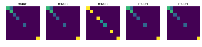
• 13: “muon”
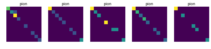
• 211: “pion”
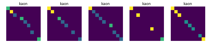
• 321: “kaon”
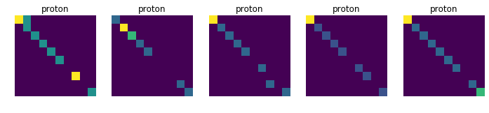
• 2212: “proton”

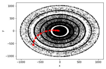
Fig 1 Transverse plane of the TrackML detector with the particle in red

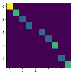
Fig 2 Translated particle with RZ binning

Files available :

• The training data consists of 350 .pkl files, each representing a unique event (or collision). Each .pkl file contains two columns: Column 1 is a list of 10x10 images. Column 2 is the particle type associated to the image (int). Training data can be downloaded at: https://cernbox.cern.ch/index.php/s/OH9tOo8VHYpHJDl. This data is open-source data.
• SampleSubmission.csv - is an example of what your submission file should look like.
• Data_test_file.pkl is the test set which contains about 4,000 images of particles (not associated with any specific event)
• cirtaChallenge.ipynb: is a starter python notebook. It shows you how to open and view a .pkl file and starts you off with a simple classifier.

Note that the training set is highly imbalanced, but the test set has been designed to be balanced.

---

First insight

#Import libraries to load and process data
import numpy as np
import pandas as pd

import matplotlib.pyplot as plt
import seaborn as sns

import pickle
import glob
import random
import os

import warnings
warnings.filterwarnings('ignore')

This dictionnary will be usefull later when we’ll need to have the meaning of each class and to know what it corresponds to.

# code to particle name dictionary : 
dic_types = {11: "electron", 13: "muon", 211: "pion", 321: "kaon", 2212: "proton"}

Let’s load only one of the binary file of the data set and see the shape :

# load a pickle file
event = pickle.load(open('../../Desktop/particle_train_data/event1.pkl', 'rb'))

# get the data and target
data, target = event[0], event[1]
target = target.astype('int')
event.shape, data.shape, target.shape, data[0].shape, target[0].shape

((2, 3598), (3598,), (3598,), (10, 10), ())

data[3597]

array([[2., 0., 0., 0., 0., 0., 0., 0., 0., 0.],
       [0., 3., 0., 0., 0., 0., 0., 0., 0., 0.],
       [0., 0., 2., 0., 0., 0., 0., 0., 0., 0.],
       [0., 0., 0., 0., 0., 0., 0., 0., 0., 0.],
       [0., 0., 0., 0., 1., 0., 0., 0., 0., 0.],
       [0., 0., 0., 0., 0., 1., 0., 0., 0., 0.],
       [0., 0., 0., 0., 0., 0., 1., 0., 0., 0.],
       [0., 0., 0., 0., 0., 0., 0., 0., 0., 0.],
       [0., 0., 0., 0., 0., 0., 0., 0., 1., 0.],
       [0., 0., 0., 0., 0., 0., 0., 0., 0., 1.]])

target[3597]

2212

target.dtype, data.dtype

(dtype(‘int32’), dtype(‘O’))

target[0].dtype, data[0].dtype

(dtype(‘int32’), dtype(‘float64’))

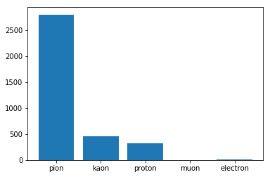
Distribution of particles in an event

We can immediately see that the target in highly imbalanced and multiclass :

from collections import Counter

plt.bar(range(len(dic_types)),list(Counter(target).values()))
plt.xticks(range(len(dic_types)), [dic_types[i] for i in list(Counter(target).keys())])
plt.show()

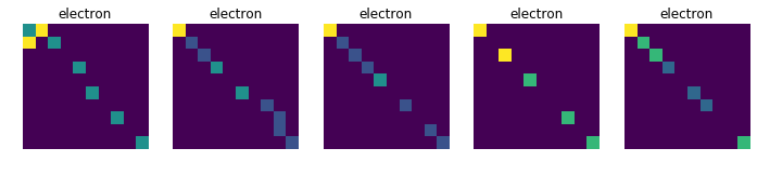
Displays 10 randomly choosen images for each collision, in order to see if there is a common pattern in each class (which is not obvious at first sight)

for j in [11, 13, 211, 321, 2212]:
    plt.figure(figsize=(12, 10))
    data_tmp = data[np.where(target==j)]
    for i in range(1, 6):
        plt.subplot(1, 5, i)
        num = random.randint(0, data_tmp.shape[0]-1)
        plt.axis('off')
        plt.title(dic_types[j])
        plt.imshow(data_tmp[num])
    plt.show()

---

Data Preparation

At first, let’s load all the data, then we have to check if all the chunks have the same shape. The second step consists in transforming all pickles files into two numpy arrays (data & target)

pkls = glob.glob('../../Desktop/particle_train_data/*.pkl')


def check_consistency():
    """Check consistency of types and shapes of the data"""
    for pk in pkls:
        event = pickle.load(open(pk, 'rb'))
        if event.shape[0] != 2:
            print("shape different for :", pk[39:-4], event.shape)
        data, target = event[0], event[1]
        target = target.astype('int')
        if data.shape != target.shape:
            print("inconsistent shapes between data & target for ", pk[39:-4], data.shape, event.shape)
        i = 0
        for d, t in zip(data, target):
            if d.dtype != 'float64' or t.dtype != 'int64':
                print("pb of type", i)
            if d.shape != (10, 10) or t.shape != ():
                print("pb of size")
            i += 1
            

def seperate_d_t(pkl):
    "load the pickle file & return flatten data & target"
    event = pickle.load(open('../../Desktop/particle_train_data/event1.pkl', 'rb'))
    data, target = event[0], event[1].astype('int')
    data = np.array([d.reshape(100) for d in data])
    return data, target


def prepare_data():
    """Merge all the pickle files"""
    # initialize the first element
    data, target = seperate_d_t('../../Desktop/particle_train_data/event1.pkl')


    # loop to concatenate the 1st with all other elts
    pkls.remove('../../Desktop/particle_train_data/event1.pkl')
    for pk in pkls:
        try:
            data_tmp, target_tmp = seperate_d_t(pk)
            data, target = np.concatenate((data, data_tmp), axis=0), np.concatenate((target, target_tmp), axis=0)
        except:
            print("pb for pk: ", pkpk[39:-4])
    return data, target
 

X_path, y_path = '../../Desktop/particle_train_data/X.csv', '../../Desktop/particle_train_data/y.csv'
        
        
# if the file are present load it instead of repreparing data        
if os.path.isfile(X_path) and os.path.isfile(y_path):
    data = np.array(pd.read_csv(X_path))
    target = np.array(pd.read_csv(y_path))
else :
    check_consistency()
    data, target = prepare_data()
    pd.DataFrame(data).to_csv(X_path, index=False)
    pd.DataFrame(target).to_csv(y_path, index=False)
    
         
data.shape, target.shape, "//", data[0].shape, target[0].shape, "//", \
data[data.shape[0]-1].shape, target[target.shape[0]-1].shape

((1259300, 100), (1259300, 1), ‘//’, (100,), (1,), ‘//’, (100,), (1,))

data[:1]

array([[3., 0., 0., 0., 0., 0., 0., 0., 0., 0., 0., 3., 0., 0., 0., 0.,
        0., 0., 0., 0., 0., 0., 1., 0., 0., 0., 0., 0., 0., 0., 0., 0.,
        0., 0., 0., 0., 0., 0., 0., 0., 0., 0., 0., 0., 1., 0., 0., 0.,
        0., 0., 0., 0., 0., 0., 0., 1., 0., 0., 0., 0., 0., 0., 0., 0.,
        0., 0., 0., 0., 0., 0., 0., 0., 0., 0., 0., 0., 0., 1., 0., 0.,
        0., 0., 0., 0., 0., 0., 0., 0., 1., 0., 0., 0., 0., 0., 0., 0.,
        0., 0., 0., 1.]])

target[:1]

array([[211]], dtype=int64)

freq = np.unique(target, return_counts=True)
freq

(array([  11,   13,  211,  321, 2212], dtype=int64),
 array([  3150,    700, 981050, 160300, 114100], dtype=int64))

Let’s compute the ratio of the least represented class :

print('ratio:', np.unique(target, return_counts=True)[1][1] / np.unique(target, return_counts=True)[1][3] * 100, '%')

ratio: 0.43668122270742354 %

---

Basic Machine Learning Models & Predictions

Now let’s use the most common and simple machine learning models in order to get a base line. As always, we need to preprocess and split our data set into a training & test parts.

Side note : it is important here to use the stratify parameter so that the proportion of values in the sample produced in our test group will be the same as the proportion of values provided to parameter stratify. This results especially useful when working around classification problems, since if we don’t provide this parameter with an array-like object, we may end with a non-representative distribution of our target classes in our test group. Furthermore, there is a class with very few records, without the stratify parameter we may have a training or a test data set without muon !

from sklearn.model_selection import train_test_split

# preprocess dataset, split into training and test part
X_train, X_test, y_train, y_test = train_test_split(data, target, test_size=0.20, random_state=42, stratify=target)
X_train.shape, X_test.shape, y_train.shape, y_test.shape

((1007440, 100), (251860, 100), (1007440, 1), (251860, 1))

from sklearn.metrics import confusion_matrix

from sklearn.tree import DecisionTreeClassifier
from sklearn.tree import ExtraTreeClassifier
from sklearn.neighbors import KNeighborsClassifier
from sklearn.linear_model import RidgeClassifier
from sklearn.ensemble import RandomForestClassifier, AdaBoostClassifier
from sklearn.svm import SVC
from sklearn.linear_model import LogisticRegression
from sklearn.svm import SVC, LinearSVC

import lightgbm as lgbm

model_list = [RandomForestClassifier(), DecisionTreeClassifier(), ExtraTreeClassifier(), RidgeClassifier(), 
             AdaBoostClassifier(), lgbm.LGBMClassifier(n_jobs = -1)]

model_names = []
train_score, test_score, f1_train, f1_test = [], [], [], []

   
def train_all_models(prefix):
    """Train all the models in the list, & fill the different lists with the predictions' scores"""
    
    # creation of list of names and scores for the train / test
    model_names_tmp = [str(m)[:str(m).index('(')] for m in model_list]
    model_names.extend([(prefix + name) for name in model_names_tmp])

    # iterate over classifiers
    for clf, name in zip(model_list, model_names_tmp):
        pickle_filename = prefix + name
        if os.path.isfile(pickle_filename):          # if model alreday been trained load it
            with open(pickle_filename, 'rb') as f:
                clf = pickle.load(f)
        else:                                        # otherwise fit model and serialize it
            clf.fit(X_train, y_train)
            with open(pickle_filename, 'wb') as f:
                pickle.dump(clf, f)          
            
        train_score.append(clf.score(X_train, y_train))
        test_score.append(clf.score(X_test, y_test))
        #print(name, f"train_score : {train_score[-1]:.2f}, test_score : {test_score[-1]:.2f}")
        
        #f1_train.append(f1_score(y_train, clf.predict(X_train)))
        #f1_test.append(f1_score(y_test, clf.predict(X_test)))
        #f1_train : {f1_train[-1]:.2f}, f1_test : {f1_test[-1]:.2f}, ")
        
        
train_all_models("1_original_data_")


def display_scores():
    """Print table & plot of all the models' scores"""
    df_score = pd.DataFrame({'model_names' : model_names,
                             'train_score' : train_score,
                             'test_score' : test_score})
    df_score = pd.melt(df_score, id_vars=['model_names'], value_vars=['train_score', 'test_score'])
    print(df_score.head(50))
    plt.figure(figsize=(12, len(model_names)/2))
    sns.barplot(y="model_names", x="value", hue="variable", data=df_score)

display_scores()

                               model_names     variable     value
0   1_original_data_RandomForestClassifier  train_score  0.902241
1   1_original_data_DecisionTreeClassifier  train_score  0.902326
2      1_original_data_ExtraTreeClassifier  train_score  0.902326
3          1_original_data_RidgeClassifier  train_score  0.783943
4       1_original_data_AdaBoostClassifier  train_score  0.577456
5           1_original_data_LGBMClassifier  train_score  0.828249
6   1_original_data_RandomForestClassifier   test_score  0.900484
7   1_original_data_DecisionTreeClassifier   test_score  0.900147
8      1_original_data_ExtraTreeClassifier   test_score  0.900147
9          1_original_data_RidgeClassifier   test_score  0.784460
10      1_original_data_AdaBoostClassifier   test_score  0.577892
11          1_original_data_LGBMClassifier   test_score  0.828194

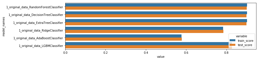
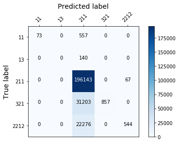
Those models aren’t effective enough, because they fail to classify correctly the least represented classes…(see the confusion matrix below). To solve this we need to rebalance the target.

---

Using the Synthetic Minority Over-sampling Technique

How SMOTe works, Brief description of the Synthetic Minority Over-sampling Technique:

It creates synthetic observations of the minority class (bad loans) by:

Finding the k-nearest-neighbors for minority class observations (finding similar observations) Randomly choosing one of the k-nearest-neighbors and using it to create a similar, but randomly tweaked, new observation. More explanations can be found here

Oversampling is a well-known way to potentially improve models trained on imbalanced data. But it’s important to remember that oversampling incorrectly can lead to thinking a model will generalize better than it actually does. Random forests are great because the model architecture reduces overfitting (see Brieman 2001 for a proof), but poor sampling practices can still lead to false conclusions about the quality of a model.

When the model is in production, it’s predicting on unseen data. The main point of model validation is to estimate how the model will generalize to new data. If the decision to put a model into production is based on how it performs on a validation set, it’s critical that oversampling is done correctly.

np.unique(y_train, return_counts=True)

(array([  11,   13,  211,  321, 2212], dtype=int64),
 array([  2516,    553, 784766, 128270,  91335], dtype=int64))

def percent_electron_muon():
    """print total nb of particules, percentage of electrons & muons, and the ratio to reach"""
    total = np.unique(y_train, return_counts=True)[1].sum()
    nb_elec = np.unique(y_train, return_counts=True)[1][0]
    nb_muon = np.unique(y_train, return_counts=True)[1][1]
    print(f"total nb of particules : {total}")
    print(f"percentage of electrons : {nb_elec/total*100:.2f}%")
    print(f"percentage of muons : {nb_muon/total*100:.2f}%")

    
percent_electron_muon()

total nb of particules : 1007440 percentage of electrons : 0.25% percentage of muons : 0.05%

# dic_types = {11: "electron", 13: "muon", 211: "pion", 321: "kaon", 2212: "proton"}
total = np.unique(y_train, return_counts=True)[1].sum()
nb_elec_goal = int(round(total*1.5/100))
nb_muon_goal = int(round(total*0.8/100))
nb_elec_goal, nb_muon_goal

(15112, 8060)

X_train, y_train = pd.DataFrame(X_train), pd.DataFrame(y_train)
X_train.shape, y_train.shape

((1007440, 100), (1007440, 1))

from imblearn.over_sampling import SMOTE

#The SMOTE is applied on the train set ONLY -When sampling_strategy is a dict, the keys correspond to the targeted classes. 
# The values correspond to the desired number of samples for each targeted class. 
# This is working for both under- and over-sampling algorithms but not for the cleaning algorithms. Use a list instead.
sm = SMOTE(sampling_strategy={11: nb_elec_goal, 13: nb_muon_goal})
X_train, y_train = sm.fit_resample(X_train, y_train)
X_train.shape, y_train.shape

((1027543, 100), (1027543,))

np.unique(y_train, return_counts=True)

(array([ 11, 13, 211, 321, 2212], dtype=int64), array([ 15112, 8060, 784766, 128270, 91335], dtype=int64))

train_all_models("2_smote_")
display_scores()

                           model_names     variable     value 0   1_original_data_RandomForestClassifier  train_score  0.902241 1   1_original_data_DecisionTreeClassifier  train_score  0.902326 2      1_original_data_ExtraTreeClassifier  train_score  0.902326 3          1_original_data_RidgeClassifier  train_score  0.783943 4       1_original_data_AdaBoostClassifier  train_score  0.577456 5           1_original_data_LGBMClassifier  train_score  0.828249 6           2_smote_RandomForestClassifier  train_score  0.900341 7           2_smote_DecisionTreeClassifier  train_score  0.900457 8              2_smote_ExtraTreeClassifier  train_score  0.900457 9                  2_smote_RidgeClassifier  train_score  0.770294 10              2_smote_AdaBoostClassifier  train_score  0.646488 11                  2_smote_LGBMClassifier  train_score  0.832237 12  1_original_data_RandomForestClassifier   test_score  0.900484 13  1_original_data_DecisionTreeClassifier   test_score  0.900147 14     1_original_data_ExtraTreeClassifier   test_score  0.900147 15         1_original_data_RidgeClassifier   test_score  0.784460 16      1_original_data_AdaBoostClassifier   test_score  0.577892 17          1_original_data_LGBMClassifier   test_score  0.828194 18          2_smote_RandomForestClassifier   test_score  0.899575 19          2_smote_DecisionTreeClassifier   test_score  0.899103 20             2_smote_ExtraTreeClassifier   test_score  0.899103 21                 2_smote_RidgeClassifier   test_score  0.784722 22              2_smote_AdaBoostClassifier   test_score  0.658695 23                  2_smote_LGBMClassifier   test_score  0.831402

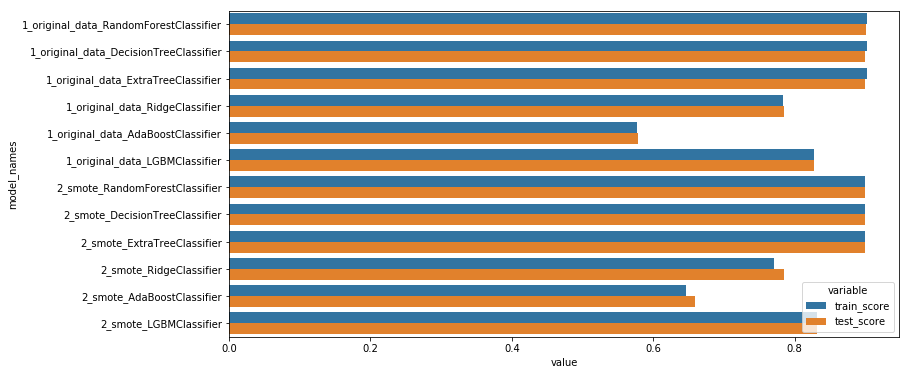
As you can see the oversampling technique doesn’t improve the result significantly. This is in fact due to the fact that i should have try different ratio. An other reason could be that those models don’t suit our needs for this particular problem… In this second part of the article (in an other blog post, you’ll see that SMOTe can indeed improve the classification results)

---

First submissions

I wasn’t able to reproduce the same metric used for this competition. And in order to see the rank of this solution, let’s submit this first results :

def train_single_model(model):
    """Train & return a single model, print score"""
    model.fit(X_train, y_train)
    print("score train", model.score(X_train, y_train))
    print("score test", model.score(X_test, y_test))
    return model


def make_submission(trained_model, csv_name):
    """Load the test pickle file, make prediction with the trained model & create a csv for submission"""
    pkl_file = open('other_data/data_test_file.pkl', 'rb')
    test = pickle.load(pkl_file)
    ss = pd.DataFrame({'image':[t[0] for t in test]})
    test_preds = trained_model.predict_proba([t[1].flatten() for t in test])
    for i in range(len(trained_model.classes_)):
      ss[trained_model.classes_[i]] = test_preds[:,i]
    ss.head()
    ss.to_csv(csv_name + '.csv', index=False)


rf = train_single_model(RandomForestClassifier(n_estimators=200, max_depth=5))
make_submission(rf, "submission_rf")

submission score = 2.95 // rank : 17th not that bad

ab_clf = train_single_model(AdaBoostClassifier(n_estimators=200))

score train 0.6194992129382441 score test 0.6183531043437205

# How well does it do?
confusion_matrix(y_test, ab_clf.predict(X_test))

array([[  2160,      0,  15320,      0,   2141],
       [     0,      0,    392,      0,      0],
       [ 30720,     74, 165417,      0,      0],
       [  4295,      0,  27765,      0,      0],
       [  3253,      0,  19506,      0,     61]], dtype=int64)

ad_final = AdaBoostClassifier(n_estimators=200).fit(X, y)
make_submission(ad_final, "submission_ab_final")

submission score : 3.87, this is worse than the 1st attempt…

rf_whole_dataset = train_single_model(RandomForestClassifier(n_estimators=200, max_depth=5)).fit(X, y)
make_submission(rf_whole_dataset, "submission_rf_whole_dataset")

score train 0.7403913453638051 score test 0.7402435965533523

submission score :2.27, this is the best score so far…

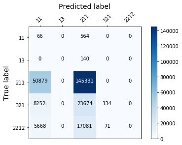
def display_confusion_matx(best_model_path):
    if os.path.isfile(best_model_path):
        with open(best_model_path, 'rb') as f:
            best_clf = pickle.load(f)
        plot_confusion_mtx(best_clf)

        
display_confusion_matx('./1_original_data_AdaBoostClassifier')

display_confusion_matx('1_original_data_LGBMClassifier')

display_confusion_matx('1_original_data_RidgeClassifier')

---

Using the Synthetic Minority Over-sampling Technique

freq_array = np.unique(y, return_counts=True)
class_weight = {k: d for k, d in zip(freq_array[0], freq_array[1])}
class_weight

{11: 3150, 13: 700, 211: 981050, 321: 160300, 2212: 114100}

tot = sum([class_weight[k] for k in class_weight])
tot

1259300

percentages = {k: round(class_weight[k] / tot * 100, 2) for k in class_weight}
percentages

{11: 0.25, 13: 0.06, 211: 77.9, 321: 12.73, 2212: 9.06}

sampling_strategy = {11: int(round(tot / 100)), 13: int(round(tot / 200))}
sampling_strategy                                                    

{11: 12593, 13: 6296}

from imblearn.over_sampling import SMOTE

#The SMOTE is applied on the train set ONLY -When sampling_strategy is a dict, the keys correspond to the targeted classes. 
# The values correspond to the desired number of samples for each targeted class. 
# This is working for both under- and over-sampling algorithms but not for the cleaning algorithms. Use a list instead.
sm = SMOTE(sampling_strategy=sampling_strategy)
X_train_smote, y_train_smote = sm.fit_resample(X_train, y_train)
pd.DataFrame(X_train_smote).to_csv('../../Desktop/particle_train_data/X_train_smote.csv', index=False)
pd.DataFrame(y_train_smote).to_csv('../../Desktop/particle_train_data/y_train_smote.csv', index=False)
X_train_smote.shape, y_train_smote.shape

((1023249, 100), (1023249,))

np.unique(y_train_smote, return_counts=True)

(array([ 11, 13, 211, 321, 2212], dtype=int64), array([ 12593, 6296, 784840, 128240, 91280], dtype=int64))

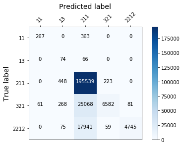
train_all_models("2_smote_")
display_confusion_matx('./2_smote_AdaBoostClassifier')

display_confusion_matx('./2_smote_LGBMClassifier')

display_confusion_matx('./2_smote_RidgeClassifier')

Randomforest with weighted classes

Let’s see if our results get better with a weight for each class !

freq_array = np.unique(y, return_counts=True)
class_weight = {k: d for k, d in zip(freq_array[0], freq_array[1])}
class_weight

rf = RandomForestClassifier(n_estimators=200, max_depth=5, n_jobs=1, class_weight=class_weight).fit(X_train, y_train)
plot_confusion_mtx(rf)

from sklearn.linear_model import LogisticRegression
from sklearn.svm import LinearSVC

logreg = LogisticRegression(n_jobs = -1).fit(X_train, y_train)
plot_confusion_mtx(logreg)

#linsvc = LinearSVC().fit(X_train, y_train)
#plot_confusion_mtx(linsvc)

np.unique(y_test, return_counts=True)

(array([ 11, 13, 211, 321, 2212], dtype=int64), array([ 630, 140, 196210, 32060, 22820], dtype=int64))

---

Using the Adasyn model

from imblearn.over_sampling import ADASYN

ad = ADASYN(sampling_strategy=sampling_strategy)
X_train_adasyn, y_train_adasyn = sm.fit_resample(X_train, y_train)
pd.DataFrame(X_train_adasyn).to_csv('../../Desktop/particle_train_data/X_train_adasyn.csv', index=False)
pd.DataFrame(y_train_adasyn).to_csv('../../Desktop/particle_train_data/y_train_adasyn.csv', index=False)
X_train_adasyn.shape, y_train_adasyn.shape

((1023249, 100), (1023249,))

np.unique(y_train_adasyn, return_counts=True)

(array([  11,   13,  211,  321, 2212], dtype=int64),
 array([ 12593,   6296, 784840, 128240,  91280], dtype=int64))

train_all_models("3_adasyn_")
display_confusion_matx('./3_adasyn_AdaBoostClassifier')

display_confusion_matx('./3_adasyn_LGBMClassifier')

display_confusion_matx('./3_adasyn_RidgeClassifier')

Partial conclusion

This is the end of the first part. After the preparation of our dataset, the different pictures recorded after a collision have been shown in order to see the new created particles. Here were used some of the most common and simple machine learning models as a base line. Even afer oversampling our data with the SMOTe technique, our results weren’t improved : the classifiers don’t recognize the least represented classes very well. To be honnest, this is a little bit disappointing, but in the second part, i’ll challenge a deep learning model with Tensorflow !