Advanced Regression Techniques to predict House Prices

Description

Ask a home buyer to describe their dream house, and they probably won’t begin with the height of the basement ceiling or the proximity to an east-west railroad. But this playground competition’s dataset proves that much more influences price negotiations than the number of bedrooms or a white-picket fence.

With 79 explanatory variables describing (almost) every aspect of residential homes in Ames, Iowa, this competition challenges you to predict the final price of each home.

Acknowledgments

The Ames Housing dataset was compiled by Dean De Cock for use in data science education. It’s an incredible alternative for data scientists looking for a modernized and expanded version of the often cited Boston Housing dataset.

Data set

Here’s a brief version of what you’ll find in the data description file.

• SalePrice - the property’s sale price in dollars. This is the target variable * that you’re trying to predict.
• MSSubClass: The building class
• MSZoning: The general zoning classification
• LotFrontage: Linear feet of street connected to property
• LotArea: Lot size in square feet
• Street: Type of road access
• Alley: Type of alley access
• LotShape: General shape of property
• LandContour: Flatness of the property
• Utilities: Type of utilities available
• LotConfig: Lot configuration
• LandSlope: Slope of property
• Neighborhood: Physical locations within Ames city limits
• Condition1: Proximity to main road or railroad
• Condition2: Proximity to main road or railroad (if a second is present)
• BldgType: Type of dwelling
• HouseStyle: Style of dwelling
• OverallQual: Overall material and finish quality
• OverallCond: Overall condition rating
• YearBuilt: Original construction date
• YearRemodAdd: Remodel date
• RoofStyle: Type of roof
• RoofMatl: Roof material
• Exterior1st: Exterior covering on house
• Exterior2nd: Exterior covering on house (if more than one material)
• MasVnrType: Masonry veneer type
• MasVnrArea: Masonry veneer area in square feet
• ExterQual: Exterior material quality
• ExterCond: Present condition of the material on the exterior
• Foundation: Type of foundation
• BsmtQual: Height of the basement
• BsmtCond: General condition of the basement
• BsmtExposure: Walkout or garden level basement walls
• BsmtFinType1: Quality of basement finished area
• BsmtFinSF1: Type 1 finished square feet
• BsmtFinType2: Quality of second finished area (if present)
• BsmtFinSF2: Type 2 finished square feet
• BsmtUnfSF: Unfinished square feet of basement area
• TotalBsmtSF: Total square feet of basement area
• Heating: Type of heating
• HeatingQC: Heating quality and condition
• CentralAir: Central air conditioning
• Electrical: Electrical system
• 1stFlrSF: First Floor square feet
• 2ndFlrSF: Second floor square feet
• LowQualFinSF: Low quality finished square feet (all floors)
• GrLivArea: Above grade (ground) living area square feet
• BsmtFullBath: Basement full bathrooms
• BsmtHalfBath: Basement half bathrooms
• FullBath: Full bathrooms above grade
• HalfBath: Half baths above grade
• Bedroom: Number of bedrooms above basement level
• Kitchen: Number of kitchens
• KitchenQual: Kitchen quality
• TotRmsAbvGrd: Total rooms above grade (does not include bathrooms)
• Functional: Home functionality rating
• Fireplaces: Number of fireplaces
• FireplaceQu: Fireplace quality
• GarageType: Garage location
• GarageYrBlt: Year garage was built
• GarageFinish: Interior finish of the garage
• GarageCars: Size of garage in car capacity
• GarageArea: Size of garage in square feet
• GarageQual: Garage quality
• GarageCond: Garage condition
• PavedDrive: Paved driveway
• WoodDeckSF: Wood deck area in square feet
• OpenPorchSF: Open porch area in square feet
• EnclosedPorch: Enclosed porch area in square feet
• 3SsnPorch: Three season porch area in square feet
• ScreenPorch: Screen porch area in square feet
• PoolArea: Pool area in square feet
• PoolQC: Pool quality
• Fence: Fence quality
• MiscFeature: Miscellaneous feature not covered in other categories
• MiscVal: USD Value of miscellaneous feature
• MoSold: Month Sold
• YrSold: Year Sold
• SaleType: Type of sale
• SaleCondition: Condition of sale

Goal

Predict sales prices and practice feature engineering, RFs, and gradient boosting Type: supervised machine learning - regression

---

Exploratory Analysis¶

import numpy as np
import pandas as pd
import matplotlib.pyplot as plt
import seaborn as sns

from sklearn.preprocessing import StandardScaler, MinMaxScaler
from sklearn.model_selection import train_test_split

# keep only relevant imports based on the regresssion or classification goals
from sklearn.metrics import mean_squared_error
from sklearn.model_selection import cross_val_score, GridSearchCV, RandomizedSearchCV

# common classifiers
#from sklearn.ensemble import RandomForestClassifier, AdaBoostClassifier
#from sklearn.linear_model import LogisticRegression, SGDClassifier
from sklearn.svm import SVC, LinearSVC

import xgboost as xgb
import lightgbm as lgbm

# common regresssors
from sklearn.linear_model import LinearRegression, Ridge, Lasso, ElasticNet, SGDRegressor, BayesianRidge
from sklearn.ensemble import RandomForestRegressor, GradientBoostingRegressor, ExtraTreesRegressor
from sklearn.svm import SVR

from sklearn.pipeline import Pipeline

# skip future warnings and display enough columns for wide data sets
import warnings
warnings.simplefilter(action='ignore') #, category=FutureWarning)
pd.set_option('display.max_columns', 100)

Data set first insight

Let’s see wath the data set looks like

df = pd.read_csv('../input/train.csv', index_col='Id' )
df.head()

	MSSubClass	MSZoning	LotFrontage	LotArea	Street	Alley	LotShape	LandContour	Utilities	LotConfig	LandSlope	Neighborhood	Condition1	Condition2	BldgType	HouseStyle	OverallQual	OverallCond	YearBuilt	YearRemodAdd	RoofStyle	RoofMatl	Exterior1st	Exterior2nd	MasVnrType	MasVnrArea	ExterQual	ExterCond	Foundation	BsmtQual	BsmtCond	BsmtExposure	BsmtFinType1	BsmtFinSF1	BsmtFinType2	BsmtFinSF2	BsmtUnfSF	TotalBsmtSF	Heating	HeatingQC	CentralAir	Electrical	1stFlrSF	2ndFlrSF	LowQualFinSF	GrLivArea	BsmtFullBath	BsmtHalfBath	FullBath	HalfBath	BedroomAbvGr	KitchenAbvGr	KitchenQual	TotRmsAbvGrd	Functional	Fireplaces	FireplaceQu	GarageType	GarageYrBlt	GarageFinish	GarageCars	GarageArea	GarageQual	GarageCond	PavedDrive	WoodDeckSF	OpenPorchSF	EnclosedPorch	3SsnPorch	ScreenPorch	PoolArea	PoolQC	Fence	MiscFeature	MiscVal	MoSold	YrSold	SaleType	SaleCondition	SalePrice
Id
1	60	RL	65.0	8450	Pave	NaN	Reg	Lvl	AllPub	Inside	Gtl	CollgCr	Norm	Norm	1Fam	2Story	7	5	2003	2003	Gable	CompShg	VinylSd	VinylSd	BrkFace	196.0	Gd	TA	PConc	Gd	TA	No	GLQ	706	Unf	0	150	856	GasA	Ex	Y	SBrkr	856	854	0	1710	1	0	2	1	3	1	Gd	8	Typ	0	NaN	Attchd	2003.0	RFn	2	548	TA	TA	Y	0	61	0	0	0	0	NaN	NaN	NaN	0	2	2008	WD	Normal	208500
2	20	RL	80.0	9600	Pave	NaN	Reg	Lvl	AllPub	FR2	Gtl	Veenker	Feedr	Norm	1Fam	1Story	6	8	1976	1976	Gable	CompShg	MetalSd	MetalSd	None	0.0	TA	TA	CBlock	Gd	TA	Gd	ALQ	978	Unf	0	284	1262	GasA	Ex	Y	SBrkr	1262	0	0	1262	0	1	2	0	3	1	TA	6	Typ	1	TA	Attchd	1976.0	RFn	2	460	TA	TA	Y	298	0	0	0	0	0	NaN	NaN	NaN	0	5	2007	WD	Normal	181500
3	60	RL	68.0	11250	Pave	NaN	IR1	Lvl	AllPub	Inside	Gtl	CollgCr	Norm	Norm	1Fam	2Story	7	5	2001	2002	Gable	CompShg	VinylSd	VinylSd	BrkFace	162.0	Gd	TA	PConc	Gd	TA	Mn	GLQ	486	Unf	0	434	920	GasA	Ex	Y	SBrkr	920	866	0	1786	1	0	2	1	3	1	Gd	6	Typ	1	TA	Attchd	2001.0	RFn	2	608	TA	TA	Y	0	42	0	0	0	0	NaN	NaN	NaN	0	9	2008	WD	Normal	223500
4	70	RL	60.0	9550	Pave	NaN	IR1	Lvl	AllPub	Corner	Gtl	Crawfor	Norm	Norm	1Fam	2Story	7	5	1915	1970	Gable	CompShg	Wd Sdng	Wd Shng	None	0.0	TA	TA	BrkTil	TA	Gd	No	ALQ	216	Unf	0	540	756	GasA	Gd	Y	SBrkr	961	756	0	1717	1	0	1	0	3	1	Gd	7	Typ	1	Gd	Detchd	1998.0	Unf	3	642	TA	TA	Y	0	35	272	0	0	0	NaN	NaN	NaN	0	2	2006	WD	Abnorml	140000
5	60	RL	84.0	14260	Pave	NaN	IR1	Lvl	AllPub	FR2	Gtl	NoRidge	Norm	Norm	1Fam	2Story	8	5	2000	2000	Gable	CompShg	VinylSd	VinylSd	BrkFace	350.0	Gd	TA	PConc	Gd	TA	Av	GLQ	655	Unf	0	490	1145	GasA	Ex	Y	SBrkr	1145	1053	0	2198	1	0	2	1	4	1	Gd	9	Typ	1	TA	Attchd	2000.0	RFn	3	836	TA	TA	Y	192	84	0	0	0	0	NaN	NaN	NaN	0	12	2008	WD	Normal	250000

Number of samples (lines) and features (colunms including the target)

df.shape

(1460, 80)

Basic infos

df.info()

<class 'pandas.core.frame.DataFrame'>
Int64Index: 1460 entries, 1 to 1460
Data columns (total 80 columns):
MSSubClass       1460 non-null int64
MSZoning         1460 non-null object
LotFrontage      1201 non-null float64
LotArea          1460 non-null int64
Street           1460 non-null object
Alley            91 non-null object
LotShape         1460 non-null object
LandContour      1460 non-null object
Utilities        1460 non-null object
LotConfig        1460 non-null object
LandSlope        1460 non-null object
Neighborhood     1460 non-null object
Condition1       1460 non-null object
Condition2       1460 non-null object
BldgType         1460 non-null object
HouseStyle       1460 non-null object
OverallQual      1460 non-null int64
OverallCond      1460 non-null int64
YearBuilt        1460 non-null int64
YearRemodAdd     1460 non-null int64
RoofStyle        1460 non-null object
RoofMatl         1460 non-null object
Exterior1st      1460 non-null object
Exterior2nd      1460 non-null object
MasVnrType       1452 non-null object
MasVnrArea       1452 non-null float64
ExterQual        1460 non-null object
ExterCond        1460 non-null object
Foundation       1460 non-null object
BsmtQual         1423 non-null object
BsmtCond         1423 non-null object
BsmtExposure     1422 non-null object
BsmtFinType1     1423 non-null object
BsmtFinSF1       1460 non-null int64
BsmtFinType2     1422 non-null object
BsmtFinSF2       1460 non-null int64
BsmtUnfSF        1460 non-null int64
TotalBsmtSF      1460 non-null int64
Heating          1460 non-null object
HeatingQC        1460 non-null object
CentralAir       1460 non-null object
Electrical       1459 non-null object
1stFlrSF         1460 non-null int64
2ndFlrSF         1460 non-null int64
LowQualFinSF     1460 non-null int64
GrLivArea        1460 non-null int64
BsmtFullBath     1460 non-null int64
BsmtHalfBath     1460 non-null int64
FullBath         1460 non-null int64
HalfBath         1460 non-null int64
BedroomAbvGr     1460 non-null int64
KitchenAbvGr     1460 non-null int64
KitchenQual      1460 non-null object
TotRmsAbvGrd     1460 non-null int64
Functional       1460 non-null object
Fireplaces       1460 non-null int64
FireplaceQu      770 non-null object
GarageType       1379 non-null object
GarageYrBlt      1379 non-null float64
GarageFinish     1379 non-null object
GarageCars       1460 non-null int64
GarageArea       1460 non-null int64
GarageQual       1379 non-null object
GarageCond       1379 non-null object
PavedDrive       1460 non-null object
WoodDeckSF       1460 non-null int64
OpenPorchSF      1460 non-null int64
EnclosedPorch    1460 non-null int64
3SsnPorch        1460 non-null int64
ScreenPorch      1460 non-null int64
PoolArea         1460 non-null int64
PoolQC           7 non-null object
Fence            281 non-null object
MiscFeature      54 non-null object
MiscVal          1460 non-null int64
MoSold           1460 non-null int64
YrSold           1460 non-null int64
SaleType         1460 non-null object
SaleCondition    1460 non-null object
SalePrice        1460 non-null int64
dtypes: float64(3), int64(34), object(43)
memory usage: 923.9+ KB

Number of columns for each type of data

df.dtypes.value_counts()

object     43
int64      34
float64     3
dtype: int64

Unique values for each type of data

df.select_dtypes('object').apply(pd.Series.nunique, axis = 0)

MSZoning          5
Street            2
Alley             2
LotShape          4
LandContour       4
Utilities         2
LotConfig         5
LandSlope         3
Neighborhood     25
Condition1        9
Condition2        8
BldgType          5
HouseStyle        8
RoofStyle         6
RoofMatl          8
Exterior1st      15
Exterior2nd      16
MasVnrType        4
ExterQual         4
ExterCond         5
Foundation        6
BsmtQual          4
BsmtCond          4
BsmtExposure      4
BsmtFinType1      6
BsmtFinType2      6
Heating           6
HeatingQC         5
CentralAir        2
Electrical        5
KitchenQual       4
Functional        7
FireplaceQu       5
GarageType        6
GarageFinish      3
GarageQual        5
GarageCond        5
PavedDrive        3
PoolQC            3
Fence             4
MiscFeature       4
SaleType          9
SaleCondition     6
dtype: int64

Ratio of missing values by column

def missing_values_table(df):
        """Function to calculate missing values by column# Funct // credits Will Koehrsen"""
    
        # Total missing values
        mis_val = df.isnull().sum()
        
        # Percentage of missing values
        mis_val_percent = 100 * df.isnull().sum() / len(df)
        
        # Make a table with the results
        mis_val_table = pd.concat([mis_val, mis_val_percent], axis=1)
        
        # Rename the columns
        mis_val_table_ren_columns = mis_val_table.rename(
        columns = {0 : 'Missing Values', 1 : '% of Total Values'})
        
        # Sort the table by percentage of missing descending
        mis_val_table_ren_columns = mis_val_table_ren_columns[
            mis_val_table_ren_columns.iloc[:,1] != 0].sort_values(
        '% of Total Values', ascending=False).round(1)
        
        # Print some summary information
        print ("Le jeu de données a " + str(df.shape[1]) + " colonnes.\n"      
            "Il y a " + str(mis_val_table_ren_columns.shape[0]) +
              " colonnes avec des valeurs manquantes.")
        
        # Return the dataframe with missing information
        return mis_val_table_ren_columns

missing_values = missing_values_table(df)
missing_values.head(10)

Le jeu de données a 80 colonnes.
Il y a 19 colonnes avec des valeurs manquantes.

	Missing Values	% of Total Values
PoolQC	1453	99.5
MiscFeature	1406	96.3
Alley	1369	93.8
Fence	1179	80.8
FireplaceQu	690	47.3
LotFrontage	259	17.7
GarageType	81	5.5
GarageYrBlt	81	5.5
GarageFinish	81	5.5
GarageQual	81	5.5

cat_feat = list(df.select_dtypes('object').columns)
num_feat = list(df.select_dtypes(exclude='object').columns)

Data Visualization

informations on the target

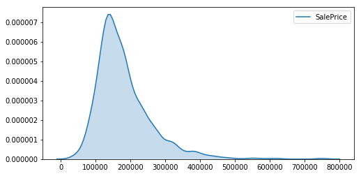
plt.figure(figsize=(8, 4))
sns.kdeplot(df.SalePrice, shade=True)
plt.show()

plt.figure(figsize=(10, 6))
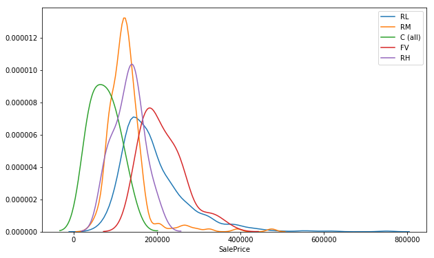
for zone in list(df.MSZoning.unique()):
    sns.distplot(df[df.MSZoning==zone].SalePrice, label=zone, hist=False)
plt.show()

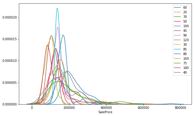
plt.figure(figsize=(10, 6))
for ms_sub_class in list(df.MSSubClass.unique()):
    sns.distplot(df[df.MSSubClass==ms_sub_class].SalePrice, label=ms_sub_class, hist=False)
plt.show()

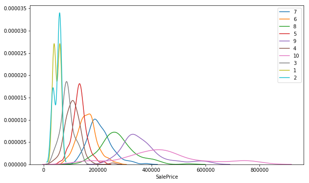
plt.figure(figsize=(10, 6))
for qual in list(df.OverallQual.unique()):
    sns.distplot(df[df.OverallQual==qual].SalePrice, label=qual, hist=False)
plt.show()

df.SalePrice.describe()

count      1460.000000
mean     180921.195890
std       79442.502883
min       34900.000000
25%      129975.000000
50%      163000.000000
75%      214000.000000
max      755000.000000
Name: SalePrice, dtype: float64

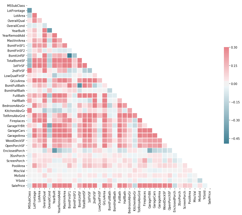
Correlations

corr = df.corr()
corr

# Generate a mask for the upper triangle
mask = np.zeros_like(corr, dtype=np.bool)
mask[np.triu_indices_from(mask)] = True

# Set up the matplotlib figure
f, ax = plt.subplots(figsize=(14, 12))

# Generate a custom diverging colormap
cmap = sns.diverging_palette(220, 10, as_cmap=True)

# Draw the heatmap with the mask and correct aspect ratio
sns.heatmap(corr, mask=mask, cmap=cmap, vmax=.3, center=0, square=True, linewidths=.5, cbar_kws={"shrink": .5}) #annot=True

<matplotlib.axes._subplots.AxesSubplot at 0x7fbbf318cfd0>

Top 50% Corralation train attributes with sale-price

top_feature = corr.index[abs(corr['SalePrice']>0.5)]
plt.subplots(figsize=(12, 8))
top_corr = df[top_feature].corr()
sns.heatmap(top_corr, annot=True)
plt.show()

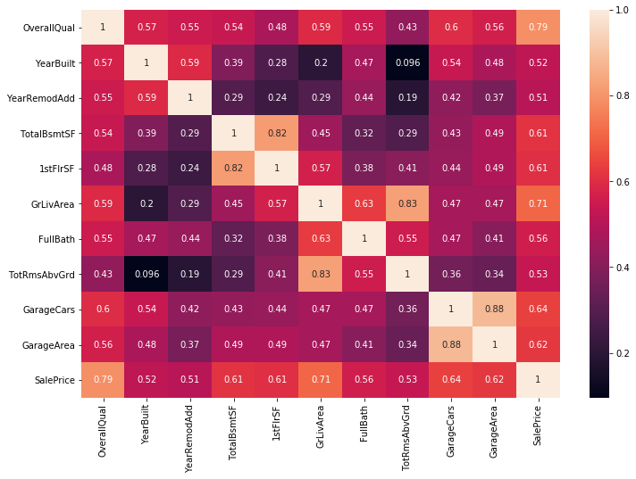
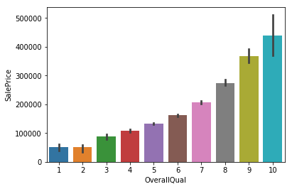
OverallQual is highly correlated with target feature of saleprice by near 80%

sns.barplot(df.OverallQual, df.SalePrice)

<matplotlib.axes._subplots.AxesSubplot at 0x7fbbf16a0550>

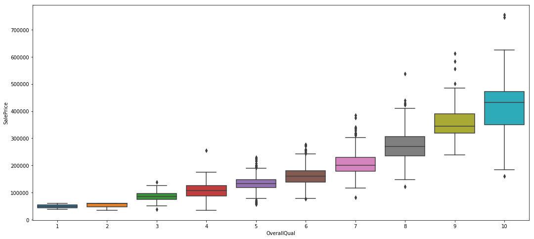
plt.figure(figsize=(18, 8))
sns.boxplot(x=df.OverallQual, y=df.SalePrice)

<matplotlib.axes._subplots.AxesSubplot at 0x7fbbf1335a20>

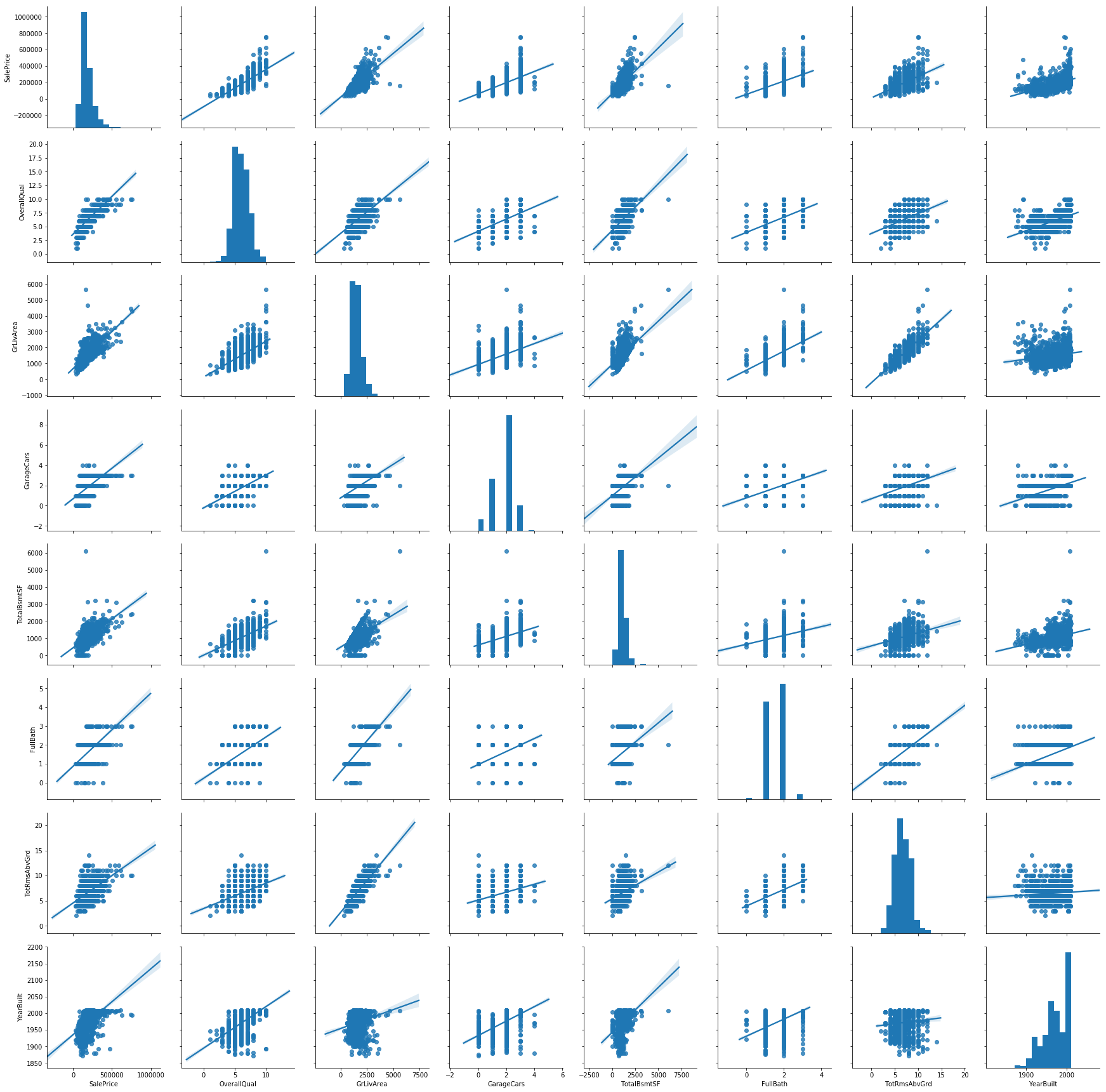
col = ['SalePrice', 'OverallQual', 'GrLivArea', 'GarageCars', 'TotalBsmtSF', 'FullBath', 'TotRmsAbvGrd', 'YearBuilt']
sns.pairplot(df[col], height=3, kind='reg')

<seaborn.axisgrid.PairGrid at 0x7fbbf1668898>

print("Most postively correlated features with the target")
corr = df.corr()
corr.sort_values(['SalePrice'], ascending=False, inplace=True)
corr.SalePrice

Most postively correlated features with the target





SalePrice        1.000000
OverallQual      0.790982
GrLivArea        0.708624
GarageCars       0.640409
GarageArea       0.623431
TotalBsmtSF      0.613581
1stFlrSF         0.605852
FullBath         0.560664
TotRmsAbvGrd     0.533723
YearBuilt        0.522897
YearRemodAdd     0.507101
GarageYrBlt      0.486362
MasVnrArea       0.477493
Fireplaces       0.466929
BsmtFinSF1       0.386420
LotFrontage      0.351799
WoodDeckSF       0.324413
2ndFlrSF         0.319334
OpenPorchSF      0.315856
HalfBath         0.284108
LotArea          0.263843
BsmtFullBath     0.227122
BsmtUnfSF        0.214479
BedroomAbvGr     0.168213
ScreenPorch      0.111447
PoolArea         0.092404
MoSold           0.046432
3SsnPorch        0.044584
BsmtFinSF2      -0.011378
BsmtHalfBath    -0.016844
MiscVal         -0.021190
LowQualFinSF    -0.025606
YrSold          -0.028923
OverallCond     -0.077856
MSSubClass      -0.084284
EnclosedPorch   -0.128578
KitchenAbvGr    -0.135907
Name: SalePrice, dtype: float64

---

Data preparation & feature engineering

Dealing with abnormal values

Not relevant here, we can assume that all values are been well integrated.

Data cleaning & Label encoding of categorical features

No duplicated rows

df.duplicated().sum()

0

Let’s remove columns with a high ratio of missing values

We don’t have much samples, so instead of removing rows with nan, missing values are then replaced by the median

from sklearn.preprocessing import LabelEncoder

def prepare_data(dataframe):

    dataframe = dataframe.drop(columns=['PoolQC', 'MiscFeature', 'Alley', 'Fence', 'FireplaceQu'])

    cat_feat = list(dataframe.select_dtypes('object').columns)
    num_feat = list(dataframe.select_dtypes(exclude='object').columns)

    dataframe[num_feat] = dataframe[num_feat].fillna(dataframe[num_feat].median())
    dataframe[cat_feat] = dataframe[cat_feat].fillna("Not communicated")
    
    for c in cat_feat:
        lbl = LabelEncoder() 
        lbl.fit(list(dataframe[c].values)) 
        dataframe[c] = lbl.transform(list(dataframe[c].values))
    
    return dataframe

At first sight, there isn’t any value in the wrong type / format

Those features can’t be used as they are (in string format), this is why we need to convert them in a numerical way…

df = prepare_data(df)

Creation of new features

• In this case, it’s complicated to add features from an other dataset because no information is provided with the CSV file we’re using.
• All columns except the id (used as index) seems to be relevant, so all of them are kept at first.
• We can also combine features to create new ones - but in this case it doesn’t seem to be really usefull.

Standardization / normalization

Not needed here

#df[num_feat] = MinMaxScaler().fit_transform(df[num_feat])

Feature selection & and data preparation for models

y = df['SalePrice']
X = df.drop(columns=['SalePrice'])
X.shape, y.shape

((1460, 74), (1460,))

Let’s split the data into a train and a test set

X_train, X_test, y_train, y_test = train_test_split(X, y, test_size=0.2)
X_train.shape, X_test.shape, y_train.shape, y_test.shape

((1168, 74), (292, 74), (1168,), (292,))

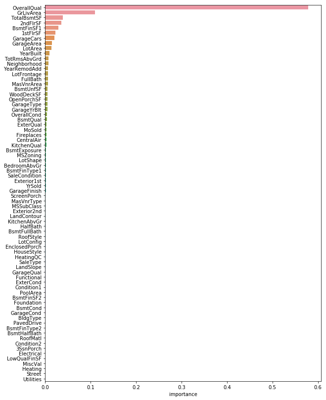
Feature importance

Top 10 most important features:

rnd_reg = RandomForestRegressor(n_estimators=500, n_jobs=-1)
rnd_reg.fit(X, y)

feature_importances = pd.DataFrame(rnd_reg.feature_importances_, index = X.columns,
                                    columns=['importance']).sort_values('importance', ascending=False)

feature_importances[:10]

	importance
OverallQual	0.578202
GrLivArea	0.109874
TotalBsmtSF	0.039231
2ndFlrSF	0.035708
BsmtFinSF1	0.029386
1stFlrSF	0.022536
GarageCars	0.020744
GarageArea	0.015562
LotArea	0.013600
YearBuilt	0.009355

Graph with features sorted by importance

plt.figure(figsize=(10, 14))
sns.barplot(x="importance", y=feature_importances.index, data=feature_importances)
plt.show()

---

Training models and results

Baselines - first selection of models

# f1_score binary by default
def get_rmse(reg, model_name):
    """Print the score for the model passed in argument and retrun scores for the train/test sets"""
    
    y_train_pred, y_pred = reg.predict(X_train), reg.predict(X_test)
    rmse_train, rmse_test = np.sqrt(mean_squared_error(y_train, y_train_pred)), np.sqrt(mean_squared_error(y_test, y_pred))
    print(model_name, f'\t - RMSE on Training  = {rmse_train:.0f} / RMSE on Test = {rmse_test:.0f}')
    
    return rmse_train, rmse_test

model_list = [
    LinearRegression(), Lasso(), SVR(),
    RandomForestRegressor(), GradientBoostingRegressor(), Ridge(), ElasticNet(), LinearSVC(),
    BayesianRidge(), ExtraTreesRegressor()
             ]

model_names = [str(m)[:str(m).index('(')] for m in model_list]
rmse_train, rmse_test = [], []

model_names

['LinearRegression',
 'Lasso',
 'SVR',
 'RandomForestRegressor',
 'GradientBoostingRegressor',
 'Ridge',
 'ElasticNet',
 'LinearSVC',
 'BayesianRidge',
 'ExtraTreesRegressor']

for model, name in zip(model_list, model_names):
    model.fit(X_train, y_train)
    sc_train, sc_test = get_rmse(model, name)
    rmse_train.append(sc_train)
    rmse_test.append(sc_test)

LinearRegression 	 - RMSE on Training  = 31163 / RMSE on Test = 32162
Lasso 	 - RMSE on Training  = 31163 / RMSE on Test = 32158
SVR 	 - RMSE on Training  = 79338 / RMSE on Test = 90251
RandomForestRegressor 	 - RMSE on Training  = 14748 / RMSE on Test = 30100
GradientBoostingRegressor 	 - RMSE on Training  = 13689 / RMSE on Test = 26783
Ridge 	 - RMSE on Training  = 31176 / RMSE on Test = 32091
ElasticNet 	 - RMSE on Training  = 32547 / RMSE on Test = 33122
LinearSVC 	 - RMSE on Training  = 94350 / RMSE on Test = 105986
BayesianRidge 	 - RMSE on Training  = 31599 / RMSE on Test = 31864
ExtraTreesRegressor 	 - RMSE on Training  = 0 / RMSE on Test = 30023

Results comparison chart

df_score = pd.DataFrame({'model_names' : model_names,
                         'rmse_train' : rmse_train,
                         'rmse_test' : rmse_test})
ax = df_score.plot.barh(y=['rmse_test', 'rmse_train'], x='model_names')

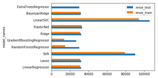
The LinearSVC model isn’t performing well because data haven’t been scaled before, let’s do it with a pipeline:

svm_reg = Pipeline([
    ("scaler", StandardScaler()),
    ("svm_regresssor", LinearSVC())
])
svm_reg.fit(X_train, y_train)
_, _ = get_rmse(svm_reg, "svr_rbf")

svr_rbf 	 - RMSE on Training  = 2158 / RMSE on Test = 70136

That’s much better, although it seems the linear kernel is the best option here:

svr_rbf = SVR(kernel = 'rbf')
svr_rbf.fit(X_train, y_train)
_, _ = get_rmse(svr_rbf, "svr_rbf")

svr_rbf 	 - RMSE on Training  = 79338 / RMSE on Test = 90251

svm_reg = Pipeline([
    ("scaler", StandardScaler()),
    ("svm_regresssor", SVR())
])
svm_reg.fit(X_train, y_train)
_, _ = get_rmse(svm_reg, "svr_rbf")

svm_reg = Pipeline([
    ("scaler", StandardScaler()),
    ("svm_regresssor", SVR(kernel="poly"))
])
svm_reg.fit(X_train, y_train)
_, _ = get_rmse(svm_reg, "svr_poly")

sgd_reg = Pipeline([
    ("scaler", StandardScaler()),
    ("sgd_regresssor", SGDRegressor())
])
sgd_reg.fit(X_train, y_train)
_, _ = get_rmse(sgd_reg, "sgd_reg") 

svr_rbf 	 - RMSE on Training  = 79310 / RMSE on Test = 90222
svr_poly 	 - RMSE on Training  = 79315 / RMSE on Test = 90224
sgd_reg 	 - RMSE on Training  = 31546 / RMSE on Test = 34055

The same remark comes true also for the SGD Regressor model

Let’s try XGBoost !

xgb_reg = xgb.XGBRegressor()
xgb_reg.fit(X_train, y_train)
_, _ = get_rmse(xgb_reg, "xgb_reg")

xgb_reg 	 - RMSE on Training  = 14601 / RMSE on Test = 27209

Looks promissing, here we can conclude that RandomForestRegressor, GradientBoostingRegressor and XGBoost seems to be the models we’ll keep for hyperparameters tuning !

Model optimisation

RandomForrestReg

from sklearn.model_selection import GridSearchCV


rf = RandomForestRegressor()
param_grid = { 
    'n_estimators': [80, 100, 120],
    'max_features': [14, 15, 16, 17],
    'max_depth' : [14, 16, 18]
}


rfc_cv = GridSearchCV(estimator=rf, param_grid=param_grid, cv=5, n_jobs=-1)
rfc_cv.fit(X_train, y_train)
print(rfc_cv.best_params_)
_, _ = get_rmse(rfc_cv, "rfc_reg")

{'max_depth': 18, 'max_features': 17, 'n_estimators': 100}
rfc_reg 	 - RMSE on Training  = 11404 / RMSE on Test = 29079

GradientBoostingReg

gb = GradientBoostingRegressor()
param_grid = { 
    'n_estimators': [100, 400],
    'max_features': [14, 15, 16, 17],
    'max_depth' : [1, 2, 8, 14, 18]
}


gb_cv = GridSearchCV(estimator=gb, param_grid=param_grid, cv=5, n_jobs=-1)
gb_cv.fit(X_train, y_train)
print(gb_cv.best_params_)
_, _ = get_rmse(gb_cv, "gb_cv")

{'max_depth': 8, 'max_features': 15, 'n_estimators': 100}
gb_cv 	 - RMSE on Training  = 1180 / RMSE on Test = 25624

XGBoostReg

xg = xgb.XGBRegressor()
param_grid = { 
    'n_estimators': [100, 400],
    'max_features': [10, 14, 16],
    'max_depth' : [1, 2, 8, 18]
}


xg_cv = GridSearchCV(estimator=xg, param_grid=param_grid, cv=5, n_jobs=-1)
xg_cv.fit(X_train, y_train)
print(xg_cv.best_params_)
_, _ = get_rmse(xg_cv, "xg_cv")

{'max_depth': 8, 'max_features': 10, 'n_estimators': 100}
xg_cv 	 - RMSE on Training  = 2478 / RMSE on Test = 28332

Combination of the best models & submission

df_test = pd.read_csv('../input/test.csv', index_col='Id' )
df_test.head()

	MSSubClass	MSZoning	LotFrontage	LotArea	Street	Alley	LotShape	LandContour	Utilities	LotConfig	LandSlope	Neighborhood	Condition1	Condition2	BldgType	HouseStyle	OverallQual	OverallCond	YearBuilt	YearRemodAdd	RoofStyle	RoofMatl	Exterior1st	Exterior2nd	MasVnrType	MasVnrArea	ExterQual	ExterCond	Foundation	BsmtQual	BsmtCond	BsmtExposure	BsmtFinType1	BsmtFinSF1	BsmtFinType2	BsmtFinSF2	BsmtUnfSF	TotalBsmtSF	Heating	HeatingQC	CentralAir	Electrical	1stFlrSF	2ndFlrSF	LowQualFinSF	GrLivArea	BsmtFullBath	BsmtHalfBath	FullBath	HalfBath	BedroomAbvGr	KitchenAbvGr	KitchenQual	TotRmsAbvGrd	Functional	Fireplaces	FireplaceQu	GarageType	GarageYrBlt	GarageFinish	GarageCars	GarageArea	GarageQual	GarageCond	PavedDrive	WoodDeckSF	OpenPorchSF	EnclosedPorch	3SsnPorch	ScreenPorch	PoolArea	PoolQC	Fence	MiscFeature	MiscVal	MoSold	YrSold	SaleType	SaleCondition
Id
1461	20	RH	80.0	11622	Pave	NaN	Reg	Lvl	AllPub	Inside	Gtl	NAmes	Feedr	Norm	1Fam	1Story	5	6	1961	1961	Gable	CompShg	VinylSd	VinylSd	None	0.0	TA	TA	CBlock	TA	TA	No	Rec	468.0	LwQ	144.0	270.0	882.0	GasA	TA	Y	SBrkr	896	0	0	896	0.0	0.0	1	0	2	1	TA	5	Typ	0	NaN	Attchd	1961.0	Unf	1.0	730.0	TA	TA	Y	140	0	0	0	120	0	NaN	MnPrv	NaN	0	6	2010	WD	Normal
1462	20	RL	81.0	14267	Pave	NaN	IR1	Lvl	AllPub	Corner	Gtl	NAmes	Norm	Norm	1Fam	1Story	6	6	1958	1958	Hip	CompShg	Wd Sdng	Wd Sdng	BrkFace	108.0	TA	TA	CBlock	TA	TA	No	ALQ	923.0	Unf	0.0	406.0	1329.0	GasA	TA	Y	SBrkr	1329	0	0	1329	0.0	0.0	1	1	3	1	Gd	6	Typ	0	NaN	Attchd	1958.0	Unf	1.0	312.0	TA	TA	Y	393	36	0	0	0	0	NaN	NaN	Gar2	12500	6	2010	WD	Normal
1463	60	RL	74.0	13830	Pave	NaN	IR1	Lvl	AllPub	Inside	Gtl	Gilbert	Norm	Norm	1Fam	2Story	5	5	1997	1998	Gable	CompShg	VinylSd	VinylSd	None	0.0	TA	TA	PConc	Gd	TA	No	GLQ	791.0	Unf	0.0	137.0	928.0	GasA	Gd	Y	SBrkr	928	701	0	1629	0.0	0.0	2	1	3	1	TA	6	Typ	1	TA	Attchd	1997.0	Fin	2.0	482.0	TA	TA	Y	212	34	0	0	0	0	NaN	MnPrv	NaN	0	3	2010	WD	Normal
1464	60	RL	78.0	9978	Pave	NaN	IR1	Lvl	AllPub	Inside	Gtl	Gilbert	Norm	Norm	1Fam	2Story	6	6	1998	1998	Gable	CompShg	VinylSd	VinylSd	BrkFace	20.0	TA	TA	PConc	TA	TA	No	GLQ	602.0	Unf	0.0	324.0	926.0	GasA	Ex	Y	SBrkr	926	678	0	1604	0.0	0.0	2	1	3	1	Gd	7	Typ	1	Gd	Attchd	1998.0	Fin	2.0	470.0	TA	TA	Y	360	36	0	0	0	0	NaN	NaN	NaN	0	6	2010	WD	Normal
1465	120	RL	43.0	5005	Pave	NaN	IR1	HLS	AllPub	Inside	Gtl	StoneBr	Norm	Norm	TwnhsE	1Story	8	5	1992	1992	Gable	CompShg	HdBoard	HdBoard	None	0.0	Gd	TA	PConc	Gd	TA	No	ALQ	263.0	Unf	0.0	1017.0	1280.0	GasA	Ex	Y	SBrkr	1280	0	0	1280	0.0	0.0	2	0	2	1	Gd	5	Typ	0	NaN	Attchd	1992.0	RFn	2.0	506.0	TA	TA	Y	0	82	0	0	144	0	NaN	NaN	NaN	0	1	2010	WD	Normal

df_test = prepare_data(df_test)
df_test.shape

(1459, 74)

rfc_sub, gb_sub, xg_sub = rfc_cv.predict(df_test), gb_cv.predict(df_test), xg_cv.predict(df_test)

sub = pd.DataFrame()
sub['Id'] = df_test.index
sub['SalePrice'] = np.mean([rfc_sub, gb_sub, xg_sub], axis=0) / 3
sub.to_csv('submission.csv',index=False)

If you found this notebook helpful or you just liked it , some upvotes would be very much appreciated - That will keep me motivated to update it on a regular basis :-)