Home Credit Default Risk Prediction

30 minute read

Predict how capable each applicant is of repaying a loan.

Context

This challenge was proposed by Home Credit Group.

Many people struggle to get loans due to insufficient or non-existent credit histories. And, unfortunately, this population is often taken advantage of by untrustworthy lenders.

Home Credit strives to broaden financial inclusion for the unbanked population by providing a positive and safe borrowing experience. In order to make sure this underserved population has a positive loan experience, Home Credit makes use of a variety of alternative data–including telco and transactional information–to predict their clients’ repayment abilities.

While Home Credit is currently using various statistical and machine learning methods to make these predictions, they’re challenging Kagglers to help them unlock the full potential of their data. Doing so will ensure that clients capable of repayment are not rejected and that loans are given with a principal, maturity, and repayment calendar that will empower their clients to be successful.

Goal

Use historical loan application data to predict whether or not an applicant will be able to repay a loan. This is a standard supervised classification task.

Submissions are evaluated on area under the ROC curve between the predicted probability and the observed target.

Type of ML

Supervised: Labels are included in the training data
Binary classification: target has only two values 0 (will repay loan on time), 1 (will have difficulty repaying loan)

Guidelines

Download and load the data
Sample the data in order to work on a smaller subset at first
Explore the data, creating functions for cleaning it
Split your data into features & labels ; training & testing
Train different models and compare performance
Train on your entire dataset, run predictions on your entire dataset and submit your results!
Iterate

Data

First insight

# usual data science stack in python
import numpy as np
import pandas as pd
import matplotlib.pyplot as plt
import seaborn as sns

import os
print(os.listdir("../input/"))

# Any results you write to the current directory are saved as output.

['application_train.csv', 'home_credit.png', 'ROC-curve.png', 'HomeCredit_columns_description_perso.csv', 'breno-assis-517356-unsplash.jpg', 'application_test.csv', 'home-credit-default-risk.zip']

# imports of need modules in sklearn
from sklearn.preprocessing import StandardScaler
from sklearn.model_selection import train_test_split
from sklearn.metrics import roc_auc_score
from sklearn.model_selection import cross_val_score

from sklearn.ensemble import RandomForestClassifier

import lightgbm as lgb
import xgboost as xgb

# set options in this notebook
pd.set_option('display.max_columns', 300)

import warnings
warnings.simplefilter(action='ignore', category=FutureWarning)

path_train = os.path.join('..', 'input', 'application_train.csv')
path_test = os.path.join('..', 'input', 'application_test.csv')

# load main datasets
app_train, app_test = pd.read_csv(path_train), pd.read_csv(path_test)

# 1st insight
app_train.tail()

	SK_ID_CURR	TARGET	NAME_CONTRACT_TYPE	CODE_GENDER	FLAG_OWN_CAR	FLAG_OWN_REALTY	AMT_INCOME_TOTAL	AMT_CREDIT	AMT_ANNUITY	AMT_GOODS_PRICE	NAME_TYPE_SUITE	NAME_INCOME_TYPE	NAME_EDUCATION_TYPE	NAME_FAMILY_STATUS	NAME_HOUSING_TYPE	REGION_POPULATION_RELATIVE	DAYS_BIRTH	DAYS_EMPLOYED	DAYS_REGISTRATION	DAYS_ID_PUBLISH	OWN_CAR_AGE	FLAG_MOBIL	FLAG_EMP_PHONE	FLAG_WORK_PHONE	FLAG_CONT_MOBILE	FLAG_PHONE	FLAG_EMAIL	OCCUPATION_TYPE	CNT_FAM_MEMBERS	REGION_RATING_CLIENT	REGION_RATING_CLIENT_W_CITY	WEEKDAY_APPR_PROCESS_START	HOUR_APPR_PROCESS_START	REG_CITY_NOT_LIVE_CITY	REG_CITY_NOT_WORK_CITY	LIVE_CITY_NOT_WORK_CITY	ORGANIZATION_TYPE	EXT_SOURCE_1	EXT_SOURCE_2	EXT_SOURCE_3	APARTMENTS_AVG	BASEMENTAREA_AVG	YEARS_BEGINEXPLUATATION_AVG	YEARS_BUILD_AVG	COMMONAREA_AVG	ELEVATORS_AVG	ENTRANCES_AVG	FLOORSMAX_AVG	FLOORSMIN_AVG	LANDAREA_AVG	LIVINGAPARTMENTS_AVG	LIVINGAREA_AVG	NONLIVINGAPARTMENTS_AVG	NONLIVINGAREA_AVG	APARTMENTS_MODE	BASEMENTAREA_MODE	YEARS_BEGINEXPLUATATION_MODE	YEARS_BUILD_MODE	COMMONAREA_MODE	ELEVATORS_MODE	ENTRANCES_MODE	FLOORSMAX_MODE	FLOORSMIN_MODE	LANDAREA_MODE	LIVINGAPARTMENTS_MODE	LIVINGAREA_MODE	NONLIVINGAPARTMENTS_MODE	NONLIVINGAREA_MODE	APARTMENTS_MEDI	BASEMENTAREA_MEDI	YEARS_BEGINEXPLUATATION_MEDI	YEARS_BUILD_MEDI	COMMONAREA_MEDI	ELEVATORS_MEDI	ENTRANCES_MEDI	FLOORSMAX_MEDI	FLOORSMIN_MEDI	LANDAREA_MEDI	LIVINGAPARTMENTS_MEDI	LIVINGAREA_MEDI	NONLIVINGAPARTMENTS_MEDI	NONLIVINGAREA_MEDI	FONDKAPREMONT_MODE	HOUSETYPE_MODE	TOTALAREA_MODE	WALLSMATERIAL_MODE	EMERGENCYSTATE_MODE	OBS_30_CNT_SOCIAL_CIRCLE	OBS_60_CNT_SOCIAL_CIRCLE	DAYS_LAST_PHONE_CHANGE	FLAG_DOCUMENT_3	FLAG_DOCUMENT_8	AMT_REQ_CREDIT_BUREAU_HOUR	AMT_REQ_CREDIT_BUREAU_DAY	AMT_REQ_CREDIT_BUREAU_WEEK	AMT_REQ_CREDIT_BUREAU_MON	AMT_REQ_CREDIT_BUREAU_QRT	AMT_REQ_CREDIT_BUREAU_YEAR
307506	456251	0	Cash loans	M	N	N	157500.0	254700.0	27558.0	225000.0	Unaccompanied	Working	Secondary / secondary special	Separated	With parents	0.032561	-9327	-236	-8456.0	-1982	NaN	1	1	0	1	0	0	Sales staff	1.0	1	1	THURSDAY	15	0	0	0	Services	0.145570	0.681632	NaN	0.2021	0.0887	0.9876	0.8300	0.0202	0.22	0.1034	0.6042	0.2708	0.0594	0.1484	0.1965	0.0753	0.1095	0.1008	0.0172	0.9782	0.7125	0.0172	0.0806	0.0345	0.4583	0.0417	0.0094	0.0882	0.0853	0.0	0.0125	0.2040	0.0887	0.9876	0.8323	0.0203	0.22	0.1034	0.6042	0.2708	0.0605	0.1509	0.2001	0.0757	0.1118	reg oper account	block of flats	0.2898	Stone, brick	No	0.0	0.0	-273.0	0	1	NaN	NaN	NaN	NaN	NaN	NaN
307507	456252	0	Cash loans	F	N	Y	72000.0	269550.0	12001.5	225000.0	Unaccompanied	Pensioner	Secondary / secondary special	Widow	House / apartment	0.025164	-20775	365243	-4388.0	-4090	NaN	1	0	0	1	1	0	NaN	1.0	2	2	MONDAY	8	0	0	0	XNA	NaN	0.115992	NaN	0.0247	0.0435	0.9727	0.6260	0.0022	0.00	0.1034	0.0833	0.1250	0.0579	0.0202	0.0257	0.0000	0.0000	0.0252	0.0451	0.9727	0.6406	0.0022	0.0000	0.1034	0.0833	0.1250	0.0592	0.0220	0.0267	0.0	0.0000	0.0250	0.0435	0.9727	0.6310	0.0022	0.00	0.1034	0.0833	0.1250	0.0589	0.0205	0.0261	0.0000	0.0000	reg oper account	block of flats	0.0214	Stone, brick	No	0.0	0.0	0.0	1	0	NaN	NaN	NaN	NaN	NaN	NaN
307508	456253	0	Cash loans	F	N	Y	153000.0	677664.0	29979.0	585000.0	Unaccompanied	Working	Higher education	Separated	House / apartment	0.005002	-14966	-7921	-6737.0	-5150	NaN	1	1	0	1	0	1	Managers	1.0	3	3	THURSDAY	9	0	1	1	School	0.744026	0.535722	0.218859	0.1031	0.0862	0.9816	0.7484	0.0123	0.00	0.2069	0.1667	0.2083	NaN	0.0841	0.9279	0.0000	0.0000	0.1050	0.0894	0.9816	0.7583	0.0124	0.0000	0.2069	0.1667	0.2083	NaN	0.0918	0.9667	0.0	0.0000	0.1041	0.0862	0.9816	0.7518	0.0124	0.00	0.2069	0.1667	0.2083	NaN	0.0855	0.9445	0.0000	0.0000	reg oper account	block of flats	0.7970	Panel	No	6.0	6.0	-1909.0	1	0	1.0	0.0	0.0	1.0	0.0	1.0
307509	456254	1	Cash loans	F	N	Y	171000.0	370107.0	20205.0	319500.0	Unaccompanied	Commercial associate	Secondary / secondary special	Married	House / apartment	0.005313	-11961	-4786	-2562.0	-931	NaN	1	1	0	1	0	0	Laborers	2.0	2	2	WEDNESDAY	9	1	1	0	Business Entity Type 1	NaN	0.514163	0.661024	0.0124	NaN	0.9771	NaN	NaN	NaN	0.0690	0.0417	NaN	NaN	NaN	0.0061	NaN	NaN	0.0126	NaN	0.9772	NaN	NaN	NaN	0.0690	0.0417	NaN	NaN	NaN	0.0063	NaN	NaN	0.0125	NaN	0.9771	NaN	NaN	NaN	0.0690	0.0417	NaN	NaN	NaN	0.0062	NaN	NaN	NaN	block of flats	0.0086	Stone, brick	No	0.0	0.0	-322.0	1	0	0.0	0.0	0.0	0.0	0.0	0.0
307510	456255	0	Cash loans	F	N	N	157500.0	675000.0	49117.5	675000.0	Unaccompanied	Commercial associate	Higher education	Married	House / apartment	0.046220	-16856	-1262	-5128.0	-410	NaN	1	1	1	1	1	0	Laborers	2.0	1	1	THURSDAY	20	0	1	1	Business Entity Type 3	0.734460	0.708569	0.113922	0.0742	0.0526	0.9881	NaN	0.0176	0.08	0.0690	0.3750	NaN	NaN	NaN	0.0791	NaN	0.0000	0.0756	0.0546	0.9881	NaN	0.0178	0.0806	0.0690	0.3750	NaN	NaN	NaN	0.0824	NaN	0.0000	0.0749	0.0526	0.9881	NaN	0.0177	0.08	0.0690	0.3750	NaN	NaN	NaN	0.0805	NaN	0.0000	NaN	block of flats	0.0718	Panel	No	0.0	0.0	-787.0	1	0	0.0	0.0	0.0	2.0	0.0	1.0

app_train.shape, app_test.shape

((307511, 122), (48744, 121))

Of course, the column named ‘TARGET’ is not in the test dataset.

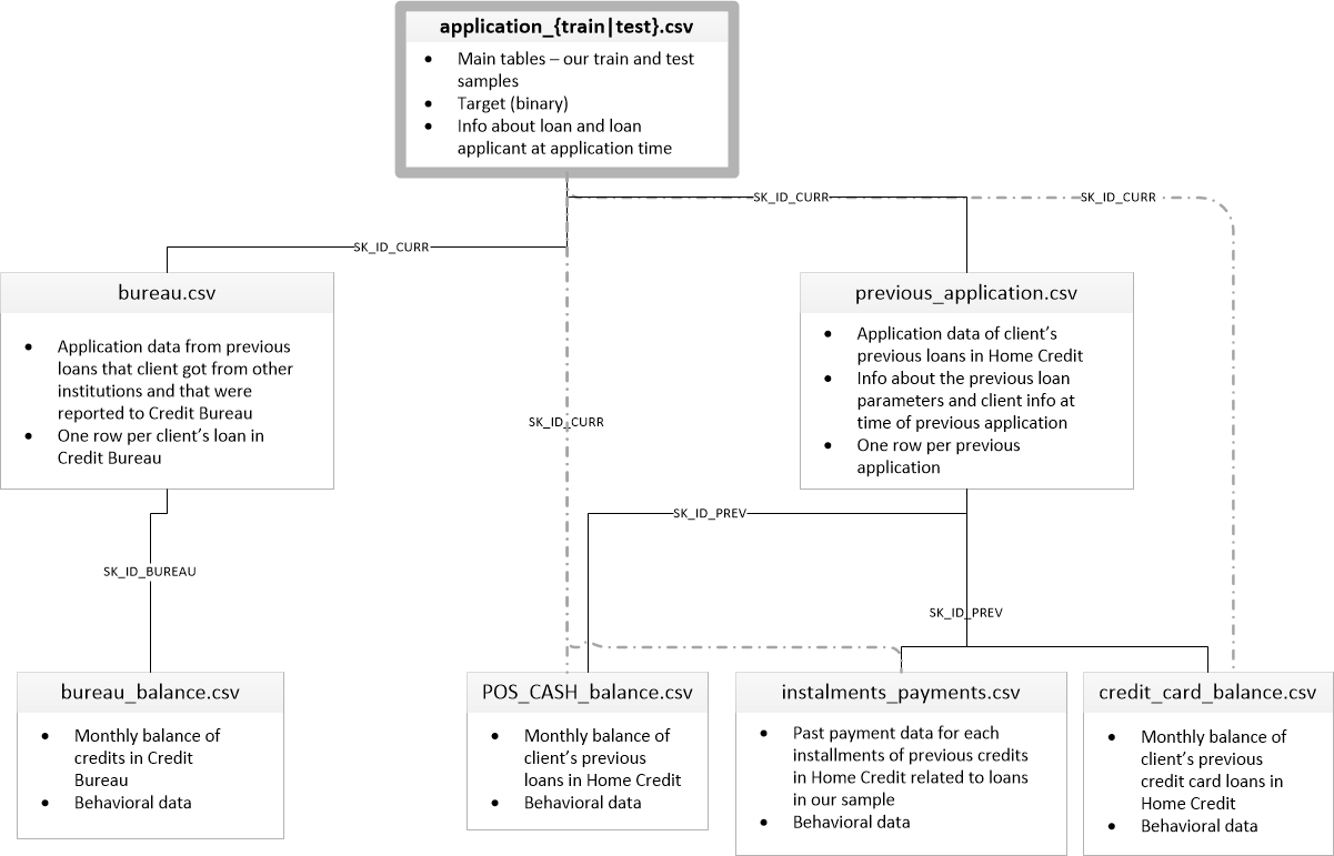
Content of each table and links between tables

_application{train test}.csv__
- This is the main table, broken into two files for Train (with TARGET) and Test (without TARGET).
- Static data for all applications. One row represents one loan in our data sample.
bureau.csv
- All client’s previous credits provided by other financial institutions that were reported to Credit Bureau (for clients who have a loan in our sample).
- For every loan in our sample, there are as many rows as number of credits the client had in Credit Bureau before the application date.
bureau_balance.csv
- Monthly balances of previous credits in Credit Bureau.
- This table has one row for each month of history of every previous credit reported to Credit Bureau – i.e the table has (#loans in sample * # of relative previous credits * # of months where we have some history observable for the previous credits) rows.
POS_CASH_balance.csv
- Monthly balance snapshots of previous POS (point of sales) and cash loans that the applicant had with Home Credit.
- This table has one row for each month of history of every previous credit in Home Credit (consumer credit and cash loans) related to loans in our sample – i.e. the table has (#loans in sample * # of relative previous credits * # of months in which we have some history observable for the previous credits) rows.
credit_card_balance.csv
- Monthly balance snapshots of previous credit cards that the applicant has with Home Credit.
- This table has one row for each month of history of every previous credit in Home Credit (consumer credit and cash loans) related to loans in our sample – i.e. the table has (#loans in sample * # of relative previous credit cards * # of months where we have some history observable for the previous credit card) rows.
previous_application.csv
- All previous applications for Home Credit loans of clients who have loans in our sample.
- There is one row for each previous application related to loans in our data sample.
installments_payments.csv
- Repayment history for the previously disbursed credits in Home Credit related to the loans in our sample.
- There is a) one row for every payment that was made plus b) one row each for missed payment.
- One row is equivalent to one payment of one installment OR one installment corresponding to one payment of one previous Home Credit credit related to loans in our sample.
HomeCredit_columns_description.csv
- This file contains descriptions for the columns in the various data files.

png

Exploratory Data Analysis¶

Distribution of the Target Column

app_train.TARGET.value_counts()

0    282686
1     24825
Name: TARGET, dtype: int64

print(f'percentage of clients with payment difficulties: {app_train.TARGET.sum() / app_train.shape[0] * 100 :.2f}%')

percentage of clients with payment difficulties: 8.07%

plt.title('Distribution of the Target Column - 1 - client with payment difficulties / 0 - all other cases')
sns.countplot(x=app_train.TARGET, data=app_train)
plt.show()

png

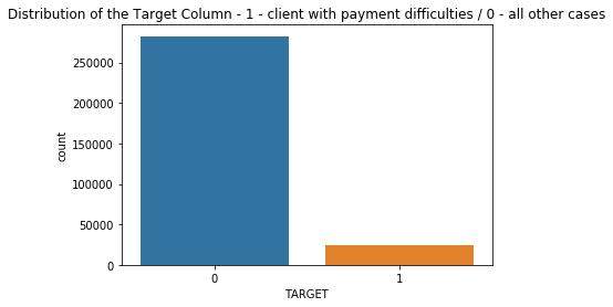
This is an imbalanced class problem. There are far more repaid loans than loans that were not repaid. It is important to weight the classes by their representation in the data to reflect this imbalance.

Column Types

app_train.dtypes.value_counts()

float64    65
int64      41
object     16
dtype: int64

int64 and float64 are numeric variables which can correspond to discrete or continuous features. Whereas object columns contain strings and are categorical features.

# Number of unique classes in each object column
app_train.select_dtypes('object').apply(pd.Series.nunique, axis=0)

NAME_CONTRACT_TYPE             2
CODE_GENDER                    3
FLAG_OWN_CAR                   2
FLAG_OWN_REALTY                2
NAME_TYPE_SUITE                7
NAME_INCOME_TYPE               8
NAME_EDUCATION_TYPE            5
NAME_FAMILY_STATUS             6
NAME_HOUSING_TYPE              6
OCCUPATION_TYPE               18
WEEKDAY_APPR_PROCESS_START     7
ORGANIZATION_TYPE             58
FONDKAPREMONT_MODE             4
HOUSETYPE_MODE                 3
WALLSMATERIAL_MODE             7
EMERGENCYSTATE_MODE            2
dtype: int64

Missing Values

# Function to calculate missing values by column# Funct // credits Will Koehrsen
def missing_values_table(df):
        # Total missing values
        mis_val = df.isnull().sum()
        
        # Percentage of missing values
        mis_val_percent = 100 * df.isnull().sum() / len(df)
        
        # Make a table with the results
        mis_val_table = pd.concat([mis_val, mis_val_percent], axis=1)
        
        # Rename the columns
        mis_val_table_ren_columns = mis_val_table.rename(
        columns = {0 : 'Missing Values', 1 : '% of Total Values'})
        
        # Sort the table by percentage of missing descending
        mis_val_table_ren_columns = mis_val_table_ren_columns[
            mis_val_table_ren_columns.iloc[:,1] != 0].sort_values(
        '% of Total Values', ascending=False).round(1)
        
        # Print some summary information
        print ("Your selected dataframe has " + str(df.shape[1]) + " columns.\n"      
            "There are " + str(mis_val_table_ren_columns.shape[0]) +
              " columns that have missing values.")
        
        # Return the dataframe with missing information
        return mis_val_table_ren_columns

# Missing values statistics
missing_values = missing_values_table(app_train)
missing_values.head(10)

Your selected dataframe has 122 columns.
There are 67 columns that have missing values.

	Missing Values	% of Total Values
COMMONAREA_MEDI	214865	69.9
COMMONAREA_AVG	214865	69.9
COMMONAREA_MODE	214865	69.9
NONLIVINGAPARTMENTS_MEDI	213514	69.4
NONLIVINGAPARTMENTS_MODE	213514	69.4
NONLIVINGAPARTMENTS_AVG	213514	69.4
FONDKAPREMONT_MODE	210295	68.4
LIVINGAPARTMENTS_MODE	210199	68.4
LIVINGAPARTMENTS_MEDI	210199	68.4
LIVINGAPARTMENTS_AVG	210199	68.4

From here we have 2 options : * Use models such as XGBoost that can handle missing values * Or drop columns with a high percentage of missing values, and fill in other columns with a low percentage It is not possible to know ahead of time if these columns will be helpful or not. My choice here is to drop them. Later if we need a more accurate score, we’ll change the way to proceed.

Dropping columns with a high ratio of missing values

# cols_to_drop = list((app_train.isnull().sum() > 75000).index)
cols_to_drop = [c for c in app_train.columns if app_train[c].isnull().sum() > 75000]

app_train, app_test = app_train.drop(cols_to_drop, axis=1), app_test.drop(cols_to_drop, axis=1)
app_test.isnull().sum().sort_values(ascending=False).head(10)

EXT_SOURCE_3                  8668
AMT_REQ_CREDIT_BUREAU_YEAR    6049
AMT_REQ_CREDIT_BUREAU_MON     6049
AMT_REQ_CREDIT_BUREAU_WEEK    6049
AMT_REQ_CREDIT_BUREAU_DAY     6049
AMT_REQ_CREDIT_BUREAU_HOUR    6049
AMT_REQ_CREDIT_BUREAU_QRT     6049
NAME_TYPE_SUITE                911
DEF_60_CNT_SOCIAL_CIRCLE        29
OBS_60_CNT_SOCIAL_CIRCLE        29
dtype: int64

Filling other missing values

obj_cols = app_train.select_dtypes('object').columns
obj_cols

Index(['NAME_CONTRACT_TYPE', 'CODE_GENDER', 'FLAG_OWN_CAR', 'FLAG_OWN_REALTY',
       'NAME_TYPE_SUITE', 'NAME_INCOME_TYPE', 'NAME_EDUCATION_TYPE',
       'NAME_FAMILY_STATUS', 'NAME_HOUSING_TYPE', 'WEEKDAY_APPR_PROCESS_START',
       'ORGANIZATION_TYPE'],
      dtype='object')

# filling string cols with 'Not specified' 
app_train[obj_cols] = app_train[obj_cols].fillna('Not specified')
app_test[obj_cols] = app_test[obj_cols].fillna('Not specified')

float_cols = app_train.select_dtypes('float').columns
float_cols

Index(['AMT_INCOME_TOTAL', 'AMT_CREDIT', 'AMT_ANNUITY', 'AMT_GOODS_PRICE',
       'REGION_POPULATION_RELATIVE', 'DAYS_REGISTRATION', 'CNT_FAM_MEMBERS',
       'EXT_SOURCE_2', 'EXT_SOURCE_3', 'OBS_30_CNT_SOCIAL_CIRCLE',
       'DEF_30_CNT_SOCIAL_CIRCLE', 'OBS_60_CNT_SOCIAL_CIRCLE',
       'DEF_60_CNT_SOCIAL_CIRCLE', 'DAYS_LAST_PHONE_CHANGE',
       'AMT_REQ_CREDIT_BUREAU_HOUR', 'AMT_REQ_CREDIT_BUREAU_DAY',
       'AMT_REQ_CREDIT_BUREAU_WEEK', 'AMT_REQ_CREDIT_BUREAU_MON',
       'AMT_REQ_CREDIT_BUREAU_QRT', 'AMT_REQ_CREDIT_BUREAU_YEAR'],
      dtype='object')

# filling float values with median of train (not test)
app_train[float_cols] = app_train[float_cols].fillna(app_train[float_cols].median())
app_test[float_cols] = app_test[float_cols].fillna(app_test[float_cols].median())

app_train.shape, app_test.shape

((307511, 72), (48744, 71))

Let’s check if there is still NaNs

app_train.isnull().sum().sort_values(ascending=False).head()

AMT_REQ_CREDIT_BUREAU_YEAR    0
AMT_REQ_CREDIT_BUREAU_QRT     0
DAYS_REGISTRATION             0
DAYS_ID_PUBLISH               0
FLAG_MOBIL                    0
dtype: int64

app_test.isnull().sum().sort_values(ascending=False).head()

AMT_REQ_CREDIT_BUREAU_YEAR    0
FLAG_EMAIL                    0
DAYS_ID_PUBLISH               0
FLAG_MOBIL                    0
FLAG_EMP_PHONE                0
dtype: int64

# Is there any duplicated rows ?

app_train.duplicated().sum()

app_test.duplicated().sum()

Categorical columns (type object)

# Number of unique classes in each object column
app_train.select_dtypes('object').apply(pd.Series.nunique, axis = 0)

NAME_CONTRACT_TYPE             2
CODE_GENDER                    3
FLAG_OWN_CAR                   2
FLAG_OWN_REALTY                2
NAME_TYPE_SUITE                8
NAME_INCOME_TYPE               8
NAME_EDUCATION_TYPE            5
NAME_FAMILY_STATUS             6
NAME_HOUSING_TYPE              6
WEEKDAY_APPR_PROCESS_START     7
ORGANIZATION_TYPE             58
dtype: int64

Dealing with anomalies

app_train['DAYS_EMPLOYED'].describe()

count    307511.000000
mean      63815.045904
std      141275.766519
min      -17912.000000
25%       -2760.000000
50%       -1213.000000
75%        -289.000000
max      365243.000000
Name: DAYS_EMPLOYED, dtype: float64

The maximum value is abnormal (besides being positive). It corresponds to 1000 years…

sns.distplot(app_train['DAYS_EMPLOYED'], kde=False);
plt.show()

png

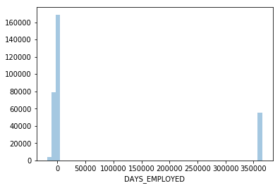
print('The non-anomalies default on %0.2f%% of loans' % (100 * app_train[app_train['DAYS_EMPLOYED'] != 365243]['TARGET'].mean()))
print('The anomalies default on %0.2f%% of loans' % (100 * app_train[app_train['DAYS_EMPLOYED'] == 365243]['TARGET'].mean()))
print('There are %d anomalous days of employment' % len(app_train[app_train['DAYS_EMPLOYED'] == 365243]))

The non-anomalies default on 8.66% of loans
The anomalies default on 5.40% of loans
There are 55374 anomalous days of employment

It turns out that the anomalies have a lower rate of default.

The anomalous values seem to have some importance. Let’s fill in the anomalous values with not a np.nan and then create a new boolean column indicating whether or not the value was anomalous.

# Create an anomalous flag column
app_train['DAYS_EMPLOYED_ANOM'] = app_train["DAYS_EMPLOYED"] == 365243

# Replace the anomalous values with nan
app_train['DAYS_EMPLOYED'].replace({365243: np.nan}, inplace = True)

sns.distplot(app_train['DAYS_EMPLOYED'].dropna(), kde=False);

png

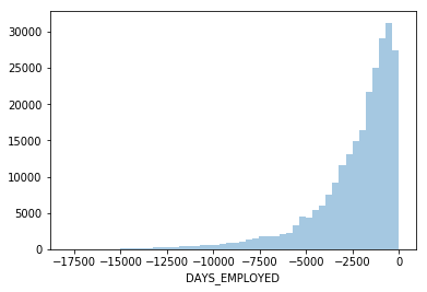
app_test['DAYS_EMPLOYED_ANOM'] = app_test["DAYS_EMPLOYED"] == 365243
app_test["DAYS_EMPLOYED"].replace({365243: np.nan}, inplace = True)

print('There are %d anomalies in the test data out of %d entries' % (app_test["DAYS_EMPLOYED_ANOM"].sum(), len(app_test)))

There are 9274 anomalies in the test data out of 48744 entries

# refilling float values with median of train (not test)

app_train[float_cols] = app_train[float_cols].apply(pd.to_numeric, errors='coerce')
app_train = app_train.fillna(app_train.median())

app_test[float_cols] = app_test[float_cols].apply(pd.to_numeric, errors='coerce')
app_test = app_train.fillna(app_test.median())

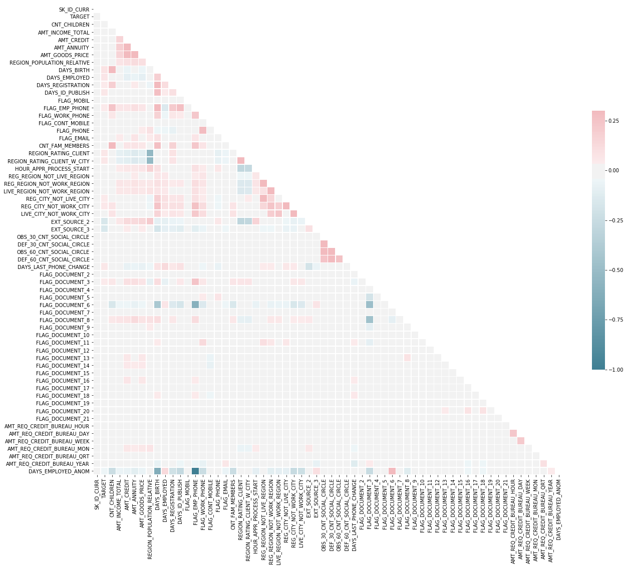
Correlations

The correlation coefficient is not the best method to represent “relevance” of a feature, but it gives us an idea of possible relationships within the data. Some general interpretations of the absolute value of the correlation coefficent are:

00-.19 “very weak”
20-.39 “weak”
40-.59 “moderate”
60-.79 “strong”
80-1.0 “very strong”

correlations = app_train.corr()['TARGET'].sort_values()

print('Most Positive Correlations:\n', correlations.tail(10))
print('\n\nMost Negative Correlations:\n', correlations.head(10))

Most Positive Correlations:
 REG_CITY_NOT_LIVE_CITY         0.044395
FLAG_EMP_PHONE                 0.045982
REG_CITY_NOT_WORK_CITY         0.050994
DAYS_ID_PUBLISH                0.051457
DAYS_LAST_PHONE_CHANGE         0.055218
REGION_RATING_CLIENT           0.058899
REGION_RATING_CLIENT_W_CITY    0.060893
DAYS_EMPLOYED                  0.063368
DAYS_BIRTH                     0.078239
TARGET                         1.000000
Name: TARGET, dtype: float64


Most Negative Correlations:
 EXT_SOURCE_2                 -0.160295
EXT_SOURCE_3                 -0.155892
DAYS_EMPLOYED_ANOM           -0.045987
AMT_GOODS_PRICE              -0.039623
REGION_POPULATION_RELATIVE   -0.037227
AMT_CREDIT                   -0.030369
FLAG_DOCUMENT_6              -0.028602
HOUR_APPR_PROCESS_START      -0.024166
FLAG_PHONE                   -0.023806
AMT_REQ_CREDIT_BUREAU_MON    -0.014794
Name: TARGET, dtype: float64

# Compute the correlation matrix
corr = app_train.corr()

# Generate a mask for the upper triangle
mask = np.zeros_like(corr, dtype=np.bool)
mask[np.triu_indices_from(mask)] = True

# Set up the matplotlib figure
f, ax = plt.subplots(figsize=(21, 19))

# Generate a custom diverging colormap
cmap = sns.diverging_palette(220, 10, as_cmap=True)

# Draw the heatmap with the mask and correct aspect ratio
sns.heatmap(corr, mask=mask, cmap=cmap, vmax=.3, center=0,
            square=True, linewidths=.5, cbar_kws={"shrink": .5})

<matplotlib.axes._subplots.AxesSubplot at 0x7f7b866f50f0>

png

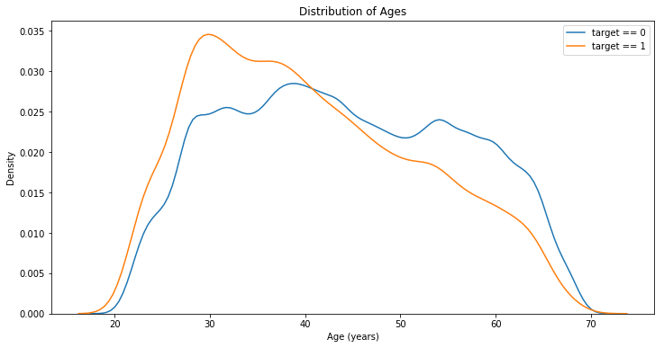
Effect of Age on Repayment

# Find the correlation of the positive days since birth and target
app_train['DAYS_BIRTH'] = abs(app_train['DAYS_BIRTH'])
app_train['DAYS_BIRTH'].corr(app_train['TARGET'])

-0.07823930830982712

There isn’t any correlation between age and repayment

plt.figure(figsize = (12, 6))

# KDE plot of loans that were repaid on time
sns.kdeplot(app_train.loc[app_train['TARGET'] == 0, 'DAYS_BIRTH'] / 365, label = 'target == 0')

# KDE plot of loans which were not repaid on time
sns.kdeplot(app_train.loc[app_train['TARGET'] == 1, 'DAYS_BIRTH'] / 365, label = 'target == 1')

# Labeling of plot
plt.xlabel('Age (years)'); plt.ylabel('Density'); plt.title('Distribution of Ages');

png

# Age information into a separate dataframe
age_data = app_train[['TARGET', 'DAYS_BIRTH']]
age_data['YEARS_BIRTH'] = age_data['DAYS_BIRTH'] / 365

# Bin the age data
age_data['YEARS_BINNED'] = pd.cut(age_data['YEARS_BIRTH'], bins = np.linspace(20, 70, num = 11))
age_data.head(10)

/home/sunflowa/anaconda3/lib/python3.7/site-packages/ipykernel_launcher.py:3: SettingWithCopyWarning: 
A value is trying to be set on a copy of a slice from a DataFrame.
Try using .loc[row_indexer,col_indexer] = value instead

See the caveats in the documentation: http://pandas.pydata.org/pandas-docs/stable/indexing.html#indexing-view-versus-copy
  This is separate from the ipykernel package so we can avoid doing imports until
/home/sunflowa/anaconda3/lib/python3.7/site-packages/ipykernel_launcher.py:6: SettingWithCopyWarning: 
A value is trying to be set on a copy of a slice from a DataFrame.
Try using .loc[row_indexer,col_indexer] = value instead

See the caveats in the documentation: http://pandas.pydata.org/pandas-docs/stable/indexing.html#indexing-view-versus-copy

	TARGET	DAYS_BIRTH	YEARS_BIRTH	YEARS_BINNED
0	1	9461	25.920548	(25.0, 30.0]
1	0	16765	45.931507	(45.0, 50.0]
2	0	19046	52.180822	(50.0, 55.0]
3	0	19005	52.068493	(50.0, 55.0]
4	0	19932	54.608219	(50.0, 55.0]
5	0	16941	46.413699	(45.0, 50.0]
6	0	13778	37.747945	(35.0, 40.0]
7	0	18850	51.643836	(50.0, 55.0]
8	0	20099	55.065753	(55.0, 60.0]
9	0	14469	39.641096	(35.0, 40.0]

# Group by the bin and calculate averages
age_groups  = age_data.groupby('YEARS_BINNED').mean()
age_groups

	TARGET	DAYS_BIRTH	YEARS_BIRTH
YEARS_BINNED
(20.0, 25.0]	0.123036	8532.795625	23.377522
(25.0, 30.0]	0.111436	10155.219250	27.822518
(30.0, 35.0]	0.102814	11854.848377	32.479037
(35.0, 40.0]	0.089414	13707.908253	37.555913
(40.0, 45.0]	0.078491	15497.661233	42.459346
(45.0, 50.0]	0.074171	17323.900441	47.462741
(50.0, 55.0]	0.066968	19196.494791	52.593136
(55.0, 60.0]	0.055314	20984.262742	57.491131
(60.0, 65.0]	0.052737	22780.547460	62.412459
(65.0, 70.0]	0.037270	24292.614340	66.555108

plt.figure(figsize = (8, 6))

# Graph the age bins and the average of the target as a bar plot
plt.bar(age_groups.index.astype(str), 100 * age_groups['TARGET'])

# Plot labeling
plt.xticks(rotation = 75); plt.xlabel('Age Group (years)'); plt.ylabel('Failure to Repay (%)')
plt.title('Failure to Repay by Age Group');

png

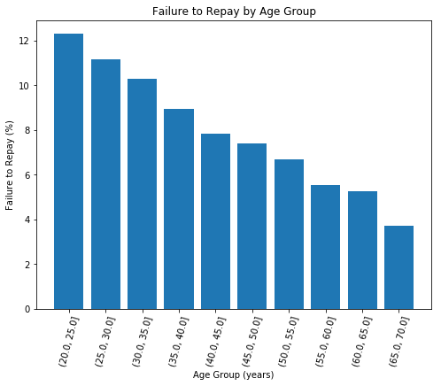
Younger applicants are more likely to not repay the loan.

Preparing data

Encoding Categorical Variables

A ML model can’t deal with categorical features (except for some models such as LightGBM). One have to find a way to encode (represent) these variables as numbers. There are two main ways :

Label encoding: assign each unique category in a categorical variable with an integer. No new columns are created. The problem with label encoding is that it gives the categories an arbitrary ordering.
One-hot encoding: create a new column for each unique category in a categorical variable. Each observation recieves a 1 in the column for its corresponding category and a 0 in all other new columns.

app_train = pd.get_dummies(data=app_train, columns=obj_cols)
app_test = pd.get_dummies(data=app_test, columns=obj_cols)

Aligning Training and Testing Data

Both the training and testing data should have the same features (columns). One-hot encoding can more columns in the one dataset because there were some categorical variables with categories not represented in the other dataset. In order to remove the columns in the training data that are not in the testing data, one need to align the dataframes.

# back up of the target /  need to keep this information
y = app_train.TARGET
app_train = app_train.drop(columns=['TARGET'])

app_train, app_test = app_train.align(app_test, join = 'inner', axis = 1)

app_train.shape, app_test.shape

((307511, 168), (307511, 168))

Scaling values

feat_to_scale = list(float_cols).copy()
feat_to_scale.extend(['CNT_CHILDREN', 'DAYS_BIRTH', 'DAYS_EMPLOYED', 'DAYS_ID_PUBLISH', 'HOUR_APPR_PROCESS_START'])
feat_to_scale

['AMT_INCOME_TOTAL',
 'AMT_CREDIT',
 'AMT_ANNUITY',
 'AMT_GOODS_PRICE',
 'REGION_POPULATION_RELATIVE',
 'DAYS_REGISTRATION',
 'CNT_FAM_MEMBERS',
 'EXT_SOURCE_2',
 'EXT_SOURCE_3',
 'OBS_30_CNT_SOCIAL_CIRCLE',
 'DEF_30_CNT_SOCIAL_CIRCLE',
 'OBS_60_CNT_SOCIAL_CIRCLE',
 'DEF_60_CNT_SOCIAL_CIRCLE',
 'DAYS_LAST_PHONE_CHANGE',
 'AMT_REQ_CREDIT_BUREAU_HOUR',
 'AMT_REQ_CREDIT_BUREAU_DAY',
 'AMT_REQ_CREDIT_BUREAU_WEEK',
 'AMT_REQ_CREDIT_BUREAU_MON',
 'AMT_REQ_CREDIT_BUREAU_QRT',
 'AMT_REQ_CREDIT_BUREAU_YEAR',
 'CNT_CHILDREN',
 'DAYS_BIRTH',
 'DAYS_EMPLOYED',
 'DAYS_ID_PUBLISH',
 'HOUR_APPR_PROCESS_START']

scaler = StandardScaler()
app_train[feat_to_scale] = scaler.fit_transform(app_train[feat_to_scale])
app_test[feat_to_scale] = scaler.fit_transform(app_test[feat_to_scale])
app_train.head()

/home/sunflowa/anaconda3/lib/python3.7/site-packages/sklearn/preprocessing/data.py:625: DataConversionWarning: Data with input dtype int64, float64 were all converted to float64 by StandardScaler.
  return self.partial_fit(X, y)
/home/sunflowa/anaconda3/lib/python3.7/site-packages/sklearn/base.py:462: DataConversionWarning: Data with input dtype int64, float64 were all converted to float64 by StandardScaler.
  return self.fit(X, **fit_params).transform(X)
/home/sunflowa/anaconda3/lib/python3.7/site-packages/sklearn/preprocessing/data.py:625: DataConversionWarning: Data with input dtype int64, float64 were all converted to float64 by StandardScaler.
  return self.partial_fit(X, y)
/home/sunflowa/anaconda3/lib/python3.7/site-packages/sklearn/base.py:462: DataConversionWarning: Data with input dtype int64, float64 were all converted to float64 by StandardScaler.
  return self.fit(X, **fit_params).transform(X)

	SK_ID_CURR	CNT_CHILDREN	AMT_INCOME_TOTAL	AMT_CREDIT	AMT_ANNUITY	AMT_GOODS_PRICE	REGION_POPULATION_RELATIVE	DAYS_BIRTH	DAYS_EMPLOYED	DAYS_REGISTRATION	DAYS_ID_PUBLISH	FLAG_MOBIL	FLAG_EMP_PHONE	FLAG_WORK_PHONE	FLAG_CONT_MOBILE	FLAG_PHONE	CNT_FAM_MEMBERS	REGION_RATING_CLIENT	REGION_RATING_CLIENT_W_CITY	HOUR_APPR_PROCESS_START	REG_CITY_NOT_WORK_CITY	LIVE_CITY_NOT_WORK_CITY	EXT_SOURCE_2	EXT_SOURCE_3	OBS_30_CNT_SOCIAL_CIRCLE	DEF_30_CNT_SOCIAL_CIRCLE	OBS_60_CNT_SOCIAL_CIRCLE	DEF_60_CNT_SOCIAL_CIRCLE	DAYS_LAST_PHONE_CHANGE	FLAG_DOCUMENT_3	FLAG_DOCUMENT_8	AMT_REQ_CREDIT_BUREAU_HOUR	AMT_REQ_CREDIT_BUREAU_DAY	AMT_REQ_CREDIT_BUREAU_WEEK	AMT_REQ_CREDIT_BUREAU_MON	AMT_REQ_CREDIT_BUREAU_QRT	AMT_REQ_CREDIT_BUREAU_YEAR	DAYS_EMPLOYED_ANOM	NAME_CONTRACT_TYPE_Cash loans	NAME_CONTRACT_TYPE_Revolving loans	CODE_GENDER_F	CODE_GENDER_M	FLAG_OWN_CAR_N	FLAG_OWN_CAR_Y	FLAG_OWN_REALTY_N	FLAG_OWN_REALTY_Y	NAME_TYPE_SUITE_Family	NAME_TYPE_SUITE_Unaccompanied	NAME_INCOME_TYPE_State servant	NAME_INCOME_TYPE_Working	NAME_EDUCATION_TYPE_Higher education	NAME_EDUCATION_TYPE_Secondary / secondary special	NAME_FAMILY_STATUS_Civil marriage	NAME_FAMILY_STATUS_Married	NAME_FAMILY_STATUS_Single / not married	NAME_HOUSING_TYPE_House / apartment	WEEKDAY_APPR_PROCESS_START_MONDAY	WEEKDAY_APPR_PROCESS_START_THURSDAY	WEEKDAY_APPR_PROCESS_START_WEDNESDAY	ORGANIZATION_TYPE_Business Entity Type 3	ORGANIZATION_TYPE_Government	ORGANIZATION_TYPE_Religion	ORGANIZATION_TYPE_School
0	100002	-0.577538	0.142129	-0.478095	-0.166143	-0.507236	-0.149452	-1.506880	0.755835	0.379837	0.579154	1	1	0	1	1	-1.265722	2	2	-0.631821	0	0	-1.317940	-2.153651	0.242861	4.163504	0.252132	5.253260	-0.206992	1	0	-0.070987	-0.058766	-0.155837	-0.269947	-0.30862	-0.440926	False	1	0	0	1	1	0	0	1	0	1	0	1	0	1	0	0	1	1	0	0	1	1	0	0	0
1	100003	-0.577538	0.426792	1.725450	0.592683	1.600873	-1.252750	0.166821	0.497899	1.078697	1.790855	1	1	0	1	1	-0.167638	1	1	-0.325620	0	0	0.564482	0.112063	-0.174085	-0.320480	-0.168527	-0.275663	0.163107	1	0	-0.070987	-0.058766	-0.155837	-0.269947	-0.30862	-1.007331	False	1	0	1	0	1	0	1	0	1	0	1	0	1	0	0	1	0	1	1	0	0	0	0	0	1
2	100004	-0.577538	-0.427196	-1.152888	-1.404669	-1.092145	-0.783451	0.689509	0.948701	0.206116	0.306869	1	1	1	1	1	-1.265722	2	2	-0.938022	0	0	0.216948	1.223975	-0.591031	-0.320480	-0.589187	-0.275663	0.178831	0	0	-0.070987	-0.058766	-0.155837	-0.269947	-0.30862	-1.007331	False	0	1	0	1	0	1	0	1	0	1	0	1	0	1	0	0	1	1	1	0	0	0	1	0	0
3	100006	-0.577538	-0.142533	-0.711430	0.177874	-0.653463	-0.928991	0.680114	-0.368597	-1.375829	0.369143	1	1	0	1	0	-0.167638	2	2	1.511587	0	0	0.712205	0.112063	0.242861	-0.320480	0.252132	-0.275663	0.418306	1	0	-0.070987	-0.058766	-0.155837	-0.269947	-0.30862	-0.440926	False	1	0	1	0	1	0	0	1	0	1	0	1	0	1	1	0	0	1	0	0	1	1	0	0	0
4	100007	-0.577538	-0.199466	-0.213734	-0.361749	-0.068554	0.563570	0.892535	-0.368129	0.191639	-0.307263	1	1	0	1	0	-1.265722	2	2	-0.325620	1	1	-1.004691	0.112063	-0.591031	-0.320480	-0.589187	-0.275663	-0.173126	0	1	-0.070987	-0.058766	-0.155837	-0.269947	-0.30862	-1.007331	False	1	0	0	1	1	0	0	1	0	1	0	1	0	1	0	0	1	1	0	1	0	0	0	1	0

Splitting training / test datasets

from app_train in order to make few predictions before submission & select models

X_train, X_test, y_train, y_test = train_test_split(app_train, y, test_size=0.2)

Base line

Metric: ROC AUC

more infos on the Receiver Operating Characteristic Area Under the Curve (ROC AUC, also sometimes called AUROC).

The Reciever Operating Characteristic (ROC) curve graphs the true positive rate versus the false positive rate:

png

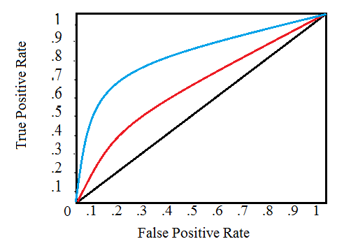
A single line on the graph indicates the curve for a single model, and movement along a line indicates changing the threshold used for classifying a positive instance. The threshold starts at 0 in the upper right to and goes to 1 in the lower left. A curve that is to the left and above another curve indicates a better model. For example, the blue model is better than the red one (which is better than the black diagonal line which indicates a naive random guessing model).

The Area Under the Curve (AUC) is the integral of the curve. This metric is between 0 and 1 with a better model scoring higher. A model that simply guesses at random will have an ROC AUC of 0.5.

When we measure a classifier according to the ROC AUC, we do not generate 0 or 1 predictions, but rather a probability between 0 and 1.

When we get into problems with inbalanced classes, accuracy is not the best metric. A model with a high ROC AUC will also have a high accuracy, but the ROC AUC is a better representation of model performance.

Random forrest

# a simple RandomForrest Classifier without CV
rf = RandomForestClassifier(n_estimators=50)
rf.fit(X_train, y_train)
y_pred = rf.predict(X_test)
roc_auc_score(y_test, y_pred)

0.5011674887648608

The predictions must be in the format shown in the sample_submission.csv file, where there are only two columns: SK_ID_CURR and TARGET. Let’s create a dataframe in this format from the test set and the predictions called submit.

def submit(model, csv_name):
    
    # fit on the whole dataset of train
    model.fit(app_train, y)
    
    # Make predictions & make sure to select the second column only
    result = model.predict_proba(app_test)[:, 1]

    submit = app_test[['SK_ID_CURR']]
    submit['TARGET'] = result

    # Save the submission to a csv file
    submit.to_csv(csv_name, index = False)

# submit(rf, 'random_forrest_clf.csv')

The random forrest model should score around 0.58329 when submitted which is not really good, because just above 0.5 i.e a random classifier…

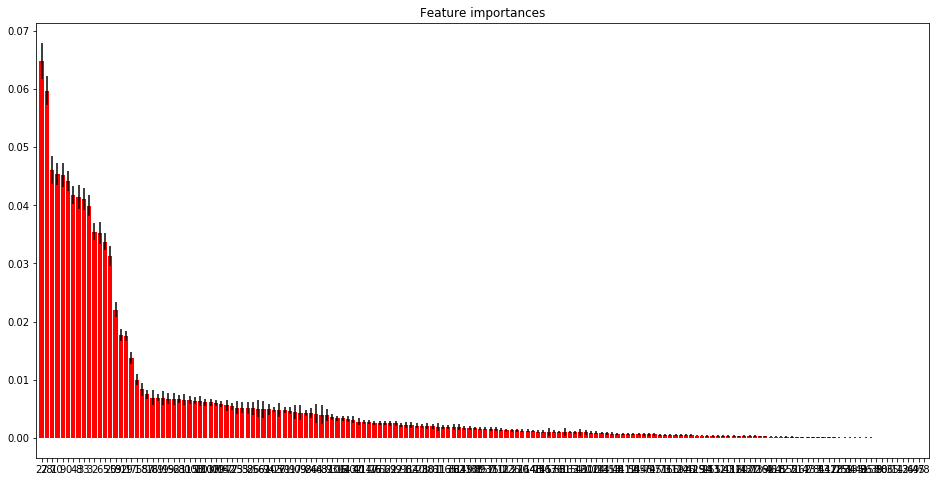
Feature Importances

importances = rf.feature_importances_
std = np.std([tree.feature_importances_ for tree in rf.estimators_], axis=0)
indices = np.argsort(importances)[::-1]

# Print the feature ranking
print("Feature ranking:")

for f in range(app_train.shape[1]):
    print("%d. feature %d (%f)" % (f + 1, indices[f], importances[indices[f]]))

Feature ranking:
feature 27 (0.064841)
feature 28 (0.059712)
feature 7 (0.046094)
feature 10 (0.045429)
feature 9 (0.045176)
feature 0 (0.044173)
feature 4 (0.041803)
feature 8 (0.041481)
feature 33 (0.041030)
feature 3 (0.039948)
feature 2 (0.035454)
feature 6 (0.035247)
feature 5 (0.033751)
feature 20 (0.031268)
feature 59 (0.022036)
feature 31 (0.017715)
feature 29 (0.017527)
feature 17 (0.013756)
feature 1 (0.010035)
feature 58 (0.008328)
feature 57 (0.007471)
feature 18 (0.006926)
feature 69 (0.006884)
feature 19 (0.006881)
feature 15 (0.006740)
feature 92 (0.006712)
feature 68 (0.006608)
feature 30 (0.006549)
feature 115 (0.006527)
feature 108 (0.006369)
feature 13 (0.006358)
feature 103 (0.006115)
feature 107 (0.006110)
feature 109 (0.006067)
feature 104 (0.005811)
feature 152 (0.005601)
feature 77 (0.005453)
feature 25 (0.005225)
feature 35 (0.005202)
feature 32 (0.005143)
feature 85 (0.005102)
feature 66 (0.004996)
feature 67 (0.004896)
feature 94 (0.004894)
feature 105 (0.004844)
feature 26 (0.004821)
feature 71 (0.004800)
feature 91 (0.004709)
feature 90 (0.004508)
feature 79 (0.004343)
feature 98 (0.004327)
feature 24 (0.004303)
feature 64 (0.004122)
feature 63 (0.004009)
feature 87 (0.003993)
feature 93 (0.003624)
feature 106 (0.003384)
feature 16 (0.003367)
feature 143 (0.003299)
feature 102 (0.003096)
feature 40 (0.002746)
feature 114 (0.002712)
feature 117 (0.002707)
feature 76 (0.002608)
feature 161 (0.002586)
feature 56 (0.002539)
feature 22 (0.002522)
feature 99 (0.002518)
feature 121 (0.002230)
feature 96 (0.002213)
feature 82 (0.002195)
feature 140 (0.002136)
feature 23 (0.002091)
feature 88 (0.002060)
feature 101 (0.001985)
feature 61 (0.001886)
feature 113 (0.001883)
feature 165 (0.001881)
feature 38 (0.001878)
feature 62 (0.001859)
feature 149 (0.001758)
feature 130 (0.001690)
feature 138 (0.001645)
feature 89 (0.001614)
feature 157 (0.001587)
feature 37 (0.001502)
feature 150 (0.001492)
feature 111 (0.001400)
feature 123 (0.001298)
feature 126 (0.001292)
feature 21 (0.001287)
feature 70 (0.001248)
feature 164 (0.001238)
feature 148 (0.001203)
feature 75 (0.001104)
feature 145 (0.001089)
feature 167 (0.001063)
feature 136 (0.001062)
feature 55 (0.001006)
feature 81 (0.001001)
feature 163 (0.000992)
feature 54 (0.000963)
feature 12 (0.000949)
feature 60 (0.000938)
feature 100 (0.000927)
feature 124 (0.000895)
feature 134 (0.000826)
feature 131 (0.000789)
feature 153 (0.000724)
feature 48 (0.000719)
feature 141 (0.000694)
feature 112 (0.000693)
feature 50 (0.000687)
feature 144 (0.000681)
feature 156 (0.000631)
feature 74 (0.000601)
feature 97 (0.000592)
feature 151 (0.000589)
feature 73 (0.000482)
feature 166 (0.000461)
feature 119 (0.000460)
feature 122 (0.000450)
feature 146 (0.000447)
feature 41 (0.000426)
feature 129 (0.000396)
feature 154 (0.000395)
feature 14 (0.000376)
feature 155 (0.000343)
feature 132 (0.000341)
feature 110 (0.000311)
feature 43 (0.000310)
feature 116 (0.000301)
feature 120 (0.000282)
feature 142 (0.000280)
feature 137 (0.000279)
feature 72 (0.000267)
feature 139 (0.000261)
feature 160 (0.000257)
feature 46 (0.000214)
feature 118 (0.000208)
feature 45 (0.000186)
feature 127 (0.000184)
feature 52 (0.000161)
feature 51 (0.000144)
feature 162 (0.000106)
feature 47 (0.000101)
feature 133 (0.000101)
feature 84 (0.000093)
feature 53 (0.000089)
feature 147 (0.000088)
feature 128 (0.000085)
feature 125 (0.000069)
feature 159 (0.000063)
feature 34 (0.000057)
feature 135 (0.000053)
feature 49 (0.000051)
feature 86 (0.000044)
feature 158 (0.000037)
feature 39 (0.000020)
feature 80 (0.000020)
feature 83 (0.000001)
feature 65 (0.000001)
feature 11 (0.000000)
feature 42 (0.000000)
feature 36 (0.000000)
feature 44 (0.000000)
feature 95 (0.000000)
feature 78 (0.000000)

# Plot the feature importances of the rf
plt.figure(figsize=(16, 8))
plt.title("Feature importances")
plt.bar(range(app_train.shape[1]), importances[indices], color="r", yerr=std[indices], align="center")
plt.xticks(range(app_train.shape[1]), indices)
plt.xlim([-1, app_train.shape[1]])
plt.show()

png

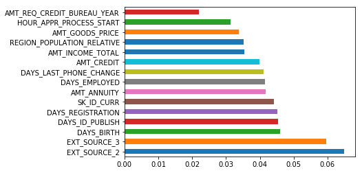
(pd.Series(rf.feature_importances_, index=app_train.columns)
   .nlargest(15)
   .plot(kind='barh'))

<matplotlib.axes._subplots.AxesSubplot at 0x7f7b8d800be0>

png

Random forrest with a cross validation

rf_cv = RandomForestClassifier()
scores = cross_val_score(rf_cv, X_train, y_train, cv=5, scoring='roc_auc', n_jobs=-1)
scores

array([0.63219173, 0.63231896, 0.62319801, 0.62533242, 0.62668538])

rf_cv.fit(X_train, y_train)
roc_auc_score(y_test, rf_cv.predict(X_test))

0.5036931060869384

#!pip install kaggle

#!kaggle competitions submit -c home-credit-default-risk -f randomforest_baseline.csv -m "My 1st submission - the baseline"

More advanced models

LightGBM

lgbm = lgb.LGBMClassifier(random_state = 50)
lgbm.fit(X_train, y_train, eval_metric = 'auc')
roc_auc_score(y_train, lgbm.predict(X_train))

0.5108945200660795

roc_auc_score(y_test, lgbm.predict(X_test))

0.5069964776833696

Different tests on hyperparameters and results:

underfitting / high biais -> let’s try to complified the model
max_depth = 7/11 or objective = ‘binary’ -> scores 0.508 / 0.508
n_estimators=1000 -> scores 0.57 / 0.511
class_weight = ‘balanced’ -> scores 0.71 / 0.68
reg_alpha = 0.1, reg_lambda = 0.1 -> no influence

lgbm = lgb.LGBMClassifier(random_state = 50, n_jobs = -1, class_weight = 'balanced')
lgbm.fit(X_train, y_train, eval_metric = 'auc')
roc_auc_score(y_train, lgbm.predict(X_train))

0.7121220817520526

roc_auc_score(y_test, lgbm.predict(X_test))

0.6846561563080866

def submit_func(model, X_Test, file_name):
    model.fit(app_train, y)
    result = model.predict_proba(app_test)[:, 1]
    submit = app_test[['SK_ID_CURR']]
    submit['TARGET'] = result
    print(submit.head())
    print(submit.shape)
    submit.to_csv(file_name + '.csv', index=False)

submit_func(lgbm, app_test, 'lgbm_submission')

/home/sunflowa/anaconda3/lib/python3.7/site-packages/ipykernel_launcher.py:5: SettingWithCopyWarning: 
A value is trying to be set on a copy of a slice from a DataFrame.
Try using .loc[row_indexer,col_indexer] = value instead

See the caveats in the documentation: http://pandas.pydata.org/pandas-docs/stable/indexing.html#indexing-view-versus-copy
  """


   SK_ID_CURR    TARGET
0      100002  0.876184
1      100003  0.237339
2      100004  0.293612
3      100006  0.427514
4      100007  0.634639
(307511, 2)

submission -> 0.72057

Using XGBoost and weighted classes

As said earlier, there are far more 0 than 1 in the target column. This is an [imbalanced class problem].(http://www.chioka.in/class-imbalance-problem/).

It’s a common problem affecting ML due to having disproportionate number of class instances in practice. This is why the ROC AUC metric suits our needs here. There are 2 class of approaches out there to deal with this problem:

1) sampling based, that can be broken into three major categories:

a) over sampling 

b) under sampling 

c) hybrid of oversampling and undersampling.

2) cost function based.

With default or few changes in hyperparameters

base score : 0.50 / 0.709
max_delta_step=2 -> unchanged
with ratio : 0.68 / 0.71

y.shape[0], y.sum()

(307511, 24825)

ratio = (y.shape[0] - y.sum()) / y.sum()
ratio

11.387150050352467

xgb_model = xgb.XGBClassifier(objective="binary:logistic", random_state=50, eval_metric='auc', 
                              max_delta_step=2, scale_pos_weight=20)
xgb_model.fit(X_train, y_train)
roc_auc_score(y_train, xgb_model.predict(X_train))

0.656946528564419

roc_auc_score(y_test, xgb_model.predict(X_test))

0.6488130660302404

For common cases when the dataset is extremely imbalanced, this can affect the training of XGBoost model, and there are two ways to improve it.

If you care only about the overall performance metric (AUC) of your prediction Balance the positive and negative weights via scale_pos_weight Use AUC for evaluation

If you care about predicting the right probability In such a case, you cannot re-balance the dataset Set parameter max_delta_step to a finite number (say 1) to help convergence

submit_func(xgb_model, app_test, 'xgb_submission')

/home/sunflowa/anaconda3/lib/python3.7/site-packages/ipykernel_launcher.py:5: SettingWithCopyWarning: 
A value is trying to be set on a copy of a slice from a DataFrame.
Try using .loc[row_indexer,col_indexer] = value instead

See the caveats in the documentation: http://pandas.pydata.org/pandas-docs/stable/indexing.html#indexing-view-versus-copy
  """


   SK_ID_CURR    TARGET
0      100002  0.908168
1      100003  0.408862
2      100004  0.452180
3      100006  0.607726
4      100007  0.763639
(307511, 2)

submission -> 0.72340

Credits / side notes

Will Koehrsen for many interesting tips in his kernel !

This notebook is intended to be an introduction to machine learning. So many things are missing or can be done better, such as :

Using function to clean / prepare the data
Exploring the other tables and select other columns that can be relevant
Doing more feature engineering, this will lead to a better score !

Twitter Facebook LinkedIn

Olivier Brunet