

How to Minimize Customer Churn
Banner made from a photo by Louis Hansel
Context
Predict behavior to retain customers. You can analyze all relevant customer data and develop focused customer retention programs.
Content
Each row represents a customer, each column contains customer’s attributes described on the column Metadata.
The data set includes information about:
- Customers who left within the last month – the column is called Churn
- Services that each customer has signed up for – phone, multiple lines, internet, online security, online backup, device protection, tech support, and streaming TV and movies
- Customer account information – how long they’ve been a customer, contract, payment method, paperless billing, monthly charges, and total charges
- Demographic info about customers – gender, age range, and if they have partners and dependents
Inspiration
To explore this type of models and learn more about the subject.
First insight
import numpy as np
import pandas as pd
import matplotlib.pyplot as plt
import seaborn as sns
from sklearn.decomposition import PCA
from sklearn.preprocessing import StandardScaler, MinMaxScaler
from sklearn.model_selection import train_test_split
from sklearn.metrics import f1_score, classification_report

from sklearn.model_selection import cross_val_score
from sklearn.ensemble import RandomForestClassifier, AdaBoostClassifier
from sklearn.linear_model import LogisticRegression, SGDClassifier
from sklearn.svm import SVC, LinearSVC
import lightgbm as lgbm
import xgboost as xgb
import warnings
warnings.simplefilter(action='ignore', category=FutureWarning)

pd.set_option('display.max_columns', 100)
df = pd.read_csv('./input/Telco-Customer-Churn.csv')
df.head()
| customerID | gender | SeniorCitizen | Partner | Dependents | tenure | PhoneService | MultipleLines | InternetService | OnlineSecurity | OnlineBackup | DeviceProtection | TechSupport | StreamingTV | StreamingMovies | Contract | PaperlessBilling | PaymentMethod | MonthlyCharges | TotalCharges | Churn | |
|---|---|---|---|---|---|---|---|---|---|---|---|---|---|---|---|---|---|---|---|---|---|
| 0 | 7590-VHVEG | Female | 0 | Yes | No | 1 | No | No phone service | DSL | No | Yes | No | No | No | No | Month-to-month | Yes | Electronic check | 29.85 | 29.85 | No |
| 1 | 5575-GNVDE | Male | 0 | No | No | 34 | Yes | No | DSL | Yes | No | Yes | No | No | No | One year | No | Mailed check | 56.95 | 1889.5 | No |
| 2 | 3668-QPYBK | Male | 0 | No | No | 2 | Yes | No | DSL | Yes | Yes | No | No | No | No | Month-to-month | Yes | Mailed check | 53.85 | 108.15 | Yes |
| 3 | 7795-CFOCW | Male | 0 | No | No | 45 | No | No phone service | DSL | Yes | No | Yes | Yes | No | No | One year | No | Bank transfer (automatic) | 42.30 | 1840.75 | No |
| 4 | 9237-HQITU | Female | 0 | No | No | 2 | Yes | No | Fiber optic | No | No | No | No | No | No | Month-to-month | Yes | Electronic check | 70.70 | 151.65 | Yes |
df.shape
(7043, 21)
The dataset contains about 7000 customers with 19 features.
Features are the following:
customerID: a unique ID for each customergender: the gender of the customerSeniorCitizen: whether the customer is a senior (i.e. older than 65) or notPartner: whether the customer has a partner or notDependents: whether the customer has people to take care of or nottenure: the number of months the customer has stayedPhoneService: whether the customer has a phone service or notMultipleLines: whether the customer has multiple telephonic lines or notInternetService: the kind of internet services the customer has (DSL, Fiber optic, no)OnlineSecurity: what online security the customer has (Yes, No, No internet service)OnlineBackup: whether the customer has online backup file system (Yes, No, No internet service)DeviceProtection: Whether the customer has device protection or not (Yes, No, No internet service)TechSupport: whether the customer has tech support or not (Yes, No, No internet service)StreamingTV: whether the customer has a streaming TV device (e.g. a TV box) or not (Yes, No, No internet service)StreamingMovies: whether the customer uses streaming movies (e.g. VOD) or not (Yes, No, No internet service)Contract: the contract term of the customer (Month-to-month, One year, Two year)PaperlessBilling: Whether the customer has electronic billing or not (Yes, No)PaymentMethod: payment method of the customer (Electronic check, Mailed check, Bank transfer (automatic), Credit card (automatic))MonthlyCharges: the amount charged to the customer monthlyTotalCharges: the total amount the customer paid
And the Target :
Churn: whether the customer left or not (Yes, No)
As you can see, many features are categorical with more than 2 values. You will have to handle this.
Take time to make a proper and complete EDA: this will help you build a better model.
Exploratory Data Analysis
Global infos on the dataset (null values, types…)
df.info()
<class 'pandas.core.frame.DataFrame'>
RangeIndex: 7043 entries, 0 to 7042
Data columns (total 21 columns):
customerID          7043 non-null object
gender              7043 non-null object
SeniorCitizen       7043 non-null int64
Partner             7043 non-null object
Dependents          7043 non-null object
tenure              7043 non-null int64
PhoneService        7043 non-null object
MultipleLines       7043 non-null object
InternetService     7043 non-null object
OnlineSecurity      7043 non-null object
OnlineBackup        7043 non-null object
DeviceProtection    7043 non-null object
TechSupport         7043 non-null object
StreamingTV         7043 non-null object
StreamingMovies     7043 non-null object
Contract            7043 non-null object
PaperlessBilling    7043 non-null object
PaymentMethod       7043 non-null object
MonthlyCharges      7043 non-null float64
TotalCharges        7043 non-null object
Churn               7043 non-null object
dtypes: float64(1), int64(2), object(18)
memory usage: 1.1+ MB
Nb of each type
df.dtypes.value_counts()
object     18
int64       2
float64     1
dtype: int64
Nb of unique value for each type
df.select_dtypes('object').apply(pd.Series.nunique, axis = 0)
customerID          7043
gender                 2
Partner                2
Dependents             2
PhoneService           2
MultipleLines          3
InternetService        3
OnlineSecurity         3
OnlineBackup           3
DeviceProtection       3
TechSupport            3
StreamingTV            3
StreamingMovies        3
Contract               3
PaperlessBilling       2
PaymentMethod          4
TotalCharges        6531
Churn                  2
dtype: int64
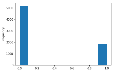
Target infos
df['Churn'].value_counts()
No     5174
Yes    1869
Name: Churn, dtype: int64
df['Churn'].str.replace('No', '0').str.replace('Yes', '1').astype(int).plot.hist()
<matplotlib.axes._subplots.AxesSubplot at 0x7f4a41ebe438>
Basic stats on numerical cols
df.describe()
| SeniorCitizen | tenure | MonthlyCharges | |
|---|---|---|---|
| count | 7043.000000 | 7043.000000 | 7043.000000 |
| mean | 0.162147 | 32.371149 | 64.761692 |
| std | 0.368612 | 24.559481 | 30.090047 |
| min | 0.000000 | 0.000000 | 18.250000 |
| 25% | 0.000000 | 9.000000 | 35.500000 |
| 50% | 0.000000 | 29.000000 | 70.350000 |
| 75% | 0.000000 | 55.000000 | 89.850000 |
| max | 1.000000 | 72.000000 | 118.750000 |
Basic cleaning
df.duplicated().sum()
0
df.isnull().sum()
customerID          0
gender              0
SeniorCitizen       0
Partner             0
Dependents          0
tenure              0
PhoneService        0
MultipleLines       0
InternetService     0
OnlineSecurity      0
OnlineBackup        0
DeviceProtection    0
TechSupport         0
StreamingTV         0
StreamingMovies     0
Contract            0
PaperlessBilling    0
PaymentMethod       0
MonthlyCharges      0
TotalCharges        0
Churn               0
dtype: int64
df = df.drop(columns=['customerID'])
No missing or duplicated rows. The customer ID is irrelevant and can be dropped.
Dealing with abnormal values
The ‘TotalCharges’ column has an object type, but it is supposed to contain only numerical values…Let’s dig a little deeper:
# example for the record strip non digit values
#test = pd.Series(["U$ 192.01"])
#test.str.replace('^[^\d]*', '').astype(float)

#df.TotalCharges = df.TotalCharges.str.replace('^[^\d]*', '')
df.iloc[0, df.columns.get_loc("TotalCharges")]
'29.85'
float(df.iloc[0, df.columns.get_loc("TotalCharges")])
29.85
df.iloc[488, df.columns.get_loc("TotalCharges")]
' '
len(df[df['TotalCharges'] == ' '])
11
Drop strange/missing values (the pandas method to_numeric could also has been used!):
# replace missing values by 0
df.TotalCharges = df.TotalCharges.replace(" ",np.nan)

# drop missing values - side note: it represents only 11 out of 7043 rows which is not significant...
df = df.dropna()

# now we can convert the column type
df.TotalCharges = df.TotalCharges.astype('float')

df.shape
(7032, 20)
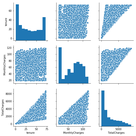
num_feat = df.select_dtypes(include=['float', 'int']).columns.tolist()
num_feat.remove('SeniorCitizen')    # SeniorCitizen is only a boolean
num_feat
['tenure', 'MonthlyCharges', 'TotalCharges']
sns.pairplot(data=df[num_feat])
plt.show()
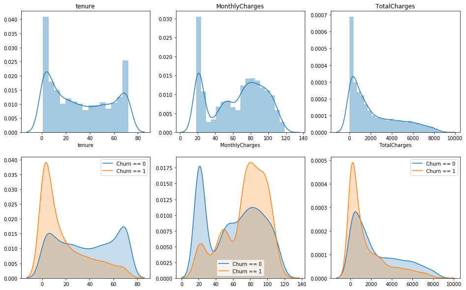
Plot distribution of those feat, w/ & w/o the distinction between the customers who churn
plt.figure(figsize=(16, 10))

plt.subplot(2, 3, 1)
sns.distplot(df['tenure'])
plt.title('tenure')

plt.subplot(2, 3, 2)
sns.distplot(df['MonthlyCharges'])
plt.title('MonthlyCharges')

plt.subplot(2, 3, 3)
sns.distplot(df['TotalCharges'])
plt.title('TotalCharges')

plt.subplot(2, 3, 4)
sns.kdeplot(df.loc[df['Churn'] == 'No', 'tenure'], shade=True,label = 'Churn == 0')
sns.kdeplot(df.loc[df['Churn'] == 'Yes', 'tenure'], shade=True,label = 'Churn == 1')

plt.subplot(2, 3, 5)
sns.kdeplot(df.loc[df['Churn'] == 'No', 'MonthlyCharges'], shade=True,label = 'Churn == 0')
sns.kdeplot(df.loc[df['Churn'] == 'Yes', 'MonthlyCharges'], shade=True,label = 'Churn == 1')

plt.subplot(2, 3, 6)
sns.kdeplot(df.loc[df['Churn'] == 'No', 'TotalCharges'], shade=True,label = 'Churn == 0')
sns.kdeplot(df.loc[df['Churn'] == 'Yes', 'TotalCharges'], shade=True,label = 'Churn == 1')
<matplotlib.axes._subplots.AxesSubplot at 0x7f4a40662e10>
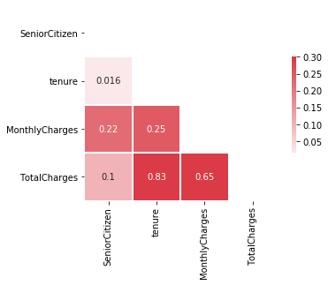
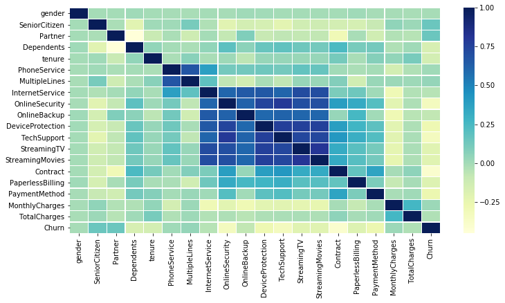
Are there any correlations ?
corr = df.corr()
corr
| SeniorCitizen | tenure | MonthlyCharges | TotalCharges | |
|---|---|---|---|---|
| SeniorCitizen | 1.000000 | 0.015683 | 0.219874 | 0.102411 |
| tenure | 0.015683 | 1.000000 | 0.246862 | 0.825880 |
| MonthlyCharges | 0.219874 | 0.246862 | 1.000000 | 0.651065 |
| TotalCharges | 0.102411 | 0.825880 | 0.651065 | 1.000000 |
# Generate a mask for the upper triangle
mask = np.zeros_like(corr, dtype=np.bool)
mask[np.triu_indices_from(mask)] = True

# Set up the matplotlib figure
f, ax = plt.subplots(figsize=(6, 4))

# Generate a custom diverging colormap
cmap = sns.diverging_palette(220, 10, as_cmap=True)

# Draw the heatmap with the mask and correct aspect ratio
sns.heatmap(corr, mask=mask, cmap=cmap, vmax=.3, center=0,
            square=True, linewidths=.5, cbar_kws={"shrink": .5}, annot=True)
<matplotlib.axes._subplots.AxesSubplot at 0x7f4a401d0da0>
plt.figure(figsize=(12, 6))

corr = df.apply(lambda x: pd.factorize(x)[0]).corr()
ax = sns.heatmap(corr, xticklabels=corr.columns, yticklabels=corr.columns,
                 linewidths=.2, cmap="YlGnBu")
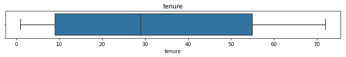
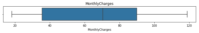
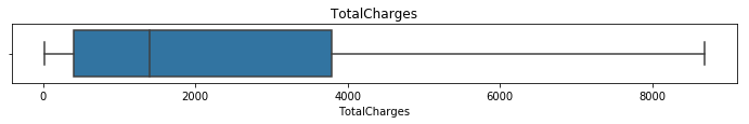
for c in num_feat:
    plt.figure(figsize=(12, 1))
    sns.boxplot(df[c])
    plt.title(c)
    plt.show()
cat_features = df.select_dtypes('object').columns.tolist()
cat_features
['gender',
 'Partner',
 'Dependents',
 'PhoneService',
 'MultipleLines',
 'InternetService',
 'OnlineSecurity',
 'OnlineBackup',
 'DeviceProtection',
 'TechSupport',
 'StreamingTV',
 'StreamingMovies',
 'Contract',
 'PaperlessBilling',
 'PaymentMethod',
 'Churn']
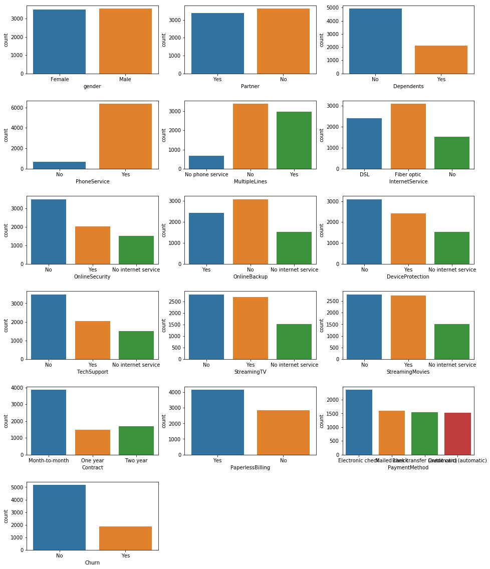
Plot the count of different categories for the other features (with text)
plt.figure(figsize=(16, 20))
plt.subplots_adjust(hspace=0.4)

for i in range(len(cat_features)):
    plt.subplot(6, 3, i+1)
    sns.countplot(df[cat_features[i]])
    #plt.title(cat_features[i])

plt.show()
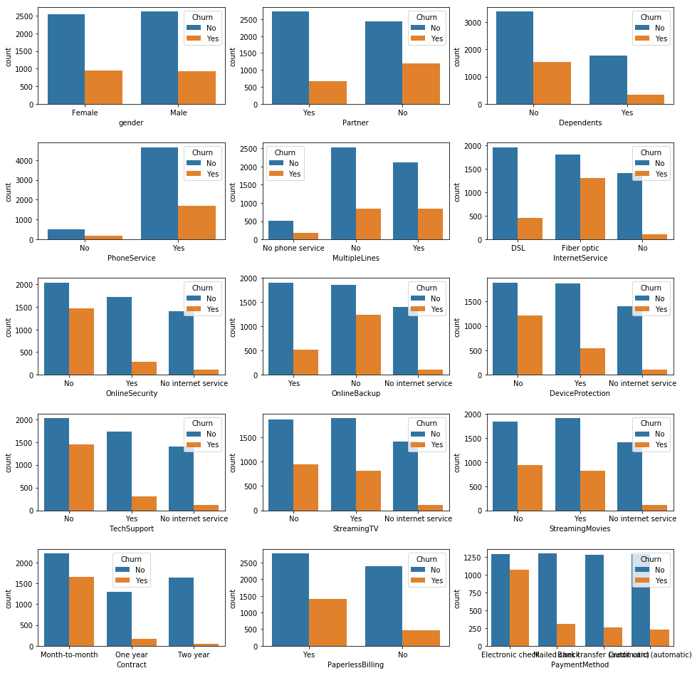
Same plot but with the distinction between customers who churn
cat_features.remove('Churn')

plt.figure(figsize=(16, 20))
plt.subplots_adjust(hspace=0.4)

for i in range(len(cat_features)):
    plt.subplot(6, 3, i+1)
    sns.countplot(df[cat_features[i]], hue=df['Churn'])
    #plt.title(cat_features[i])

plt.show()
Data Preparation & Feature engineering
Target creation
y = df.Churn.str.replace('No', '0').str.replace('Yes', '1').astype(int)
Label encoding of categorical features
X = pd.get_dummies(data=df, columns=cat_features, drop_first=True)
X = X.drop(columns=['Churn'])
X.shape, y.shape
((7032, 30), (7032,))
Features creation
- In this case, it’s complicated to add features from an other dataset because no information is provided with the CSV file we’re using.
- All columns except the user_id are relevant, so all of them are kept.
- We can combine features to create new ones : by dividing TotalCharges with the tenure which provide a kind of charge average per month. This value compared to the Monthly charges can give an idea of the charges’ evolution with time.
X['average_charges'] = X['TotalCharges'] / X['tenure']
X.loc[X['tenure'] == 0, 'average_charges'] = X['MonthlyCharges']
X.head()
| SeniorCitizen | tenure | MonthlyCharges | TotalCharges | gender_Male | Partner_Yes | Dependents_Yes | PhoneService_Yes | MultipleLines_No phone service | MultipleLines_Yes | InternetService_Fiber optic | InternetService_No | OnlineSecurity_No internet service | OnlineSecurity_Yes | OnlineBackup_No internet service | OnlineBackup_Yes | DeviceProtection_No internet service | DeviceProtection_Yes | TechSupport_No internet service | TechSupport_Yes | StreamingTV_No internet service | StreamingTV_Yes | StreamingMovies_No internet service | StreamingMovies_Yes | Contract_One year | Contract_Two year | PaperlessBilling_Yes | PaymentMethod_Credit card (automatic) | PaymentMethod_Electronic check | PaymentMethod_Mailed check | average_charges | |
|---|---|---|---|---|---|---|---|---|---|---|---|---|---|---|---|---|---|---|---|---|---|---|---|---|---|---|---|---|---|---|---|
| 0 | 0 | 1 | 29.85 | 29.85 | 0 | 1 | 0 | 0 | 1 | 0 | 0 | 0 | 0 | 0 | 0 | 1 | 0 | 0 | 0 | 0 | 0 | 0 | 0 | 0 | 0 | 0 | 1 | 0 | 1 | 0 | 29.850000 |
| 1 | 0 | 34 | 56.95 | 1889.50 | 1 | 0 | 0 | 1 | 0 | 0 | 0 | 0 | 0 | 1 | 0 | 0 | 0 | 1 | 0 | 0 | 0 | 0 | 0 | 0 | 1 | 0 | 0 | 0 | 0 | 1 | 55.573529 |
| 2 | 0 | 2 | 53.85 | 108.15 | 1 | 0 | 0 | 1 | 0 | 0 | 0 | 0 | 0 | 1 | 0 | 1 | 0 | 0 | 0 | 0 | 0 | 0 | 0 | 0 | 0 | 0 | 1 | 0 | 0 | 1 | 54.075000 |
| 3 | 0 | 45 | 42.30 | 1840.75 | 1 | 0 | 0 | 0 | 1 | 0 | 0 | 0 | 0 | 1 | 0 | 0 | 0 | 1 | 0 | 1 | 0 | 0 | 0 | 0 | 1 | 0 | 0 | 0 | 0 | 0 | 40.905556 |
| 4 | 0 | 2 | 70.70 | 151.65 | 0 | 0 | 0 | 1 | 0 | 0 | 1 | 0 | 0 | 0 | 0 | 0 | 0 | 0 | 0 | 0 | 0 | 0 | 0 | 0 | 0 | 0 | 1 | 0 | 1 | 0 | 75.825000 |
Scaling data
num_feat.append('average_charges')
scaler = MinMaxScaler()
X[num_feat] = scaler.fit_transform(X[num_feat])
/home/sunflowa/anaconda3/lib/python3.7/site-packages/sklearn/preprocessing/data.py:323: DataConversionWarning: Data with input dtype int64, float64 were all converted to float64 by MinMaxScaler.
  return self.partial_fit(X, y)
X.head()
| SeniorCitizen | tenure | MonthlyCharges | TotalCharges | gender_Male | Partner_Yes | Dependents_Yes | PhoneService_Yes | MultipleLines_No phone service | MultipleLines_Yes | InternetService_Fiber optic | InternetService_No | OnlineSecurity_No internet service | OnlineSecurity_Yes | OnlineBackup_No internet service | OnlineBackup_Yes | DeviceProtection_No internet service | DeviceProtection_Yes | TechSupport_No internet service | TechSupport_Yes | StreamingTV_No internet service | StreamingTV_Yes | StreamingMovies_No internet service | StreamingMovies_Yes | Contract_One year | Contract_Two year | PaperlessBilling_Yes | PaymentMethod_Credit card (automatic) | PaymentMethod_Electronic check | PaymentMethod_Mailed check | average_charges | |
|---|---|---|---|---|---|---|---|---|---|---|---|---|---|---|---|---|---|---|---|---|---|---|---|---|---|---|---|---|---|---|---|
| 0 | 0 | 0.000000 | 0.115423 | 0.001275 | 0 | 1 | 0 | 0 | 1 | 0 | 0 | 0 | 0 | 0 | 0 | 1 | 0 | 0 | 0 | 0 | 0 | 0 | 0 | 0 | 0 | 0 | 1 | 0 | 1 | 0 | 0.149361 |
| 1 | 0 | 0.464789 | 0.385075 | 0.215867 | 1 | 0 | 0 | 1 | 0 | 0 | 0 | 0 | 0 | 1 | 0 | 0 | 0 | 1 | 0 | 0 | 0 | 0 | 0 | 0 | 1 | 0 | 0 | 0 | 0 | 1 | 0.388372 |
| 2 | 0 | 0.014085 | 0.354229 | 0.010310 | 1 | 0 | 0 | 1 | 0 | 0 | 0 | 0 | 0 | 1 | 0 | 1 | 0 | 0 | 0 | 0 | 0 | 0 | 0 | 0 | 0 | 0 | 1 | 0 | 0 | 1 | 0.374448 |
| 3 | 0 | 0.619718 | 0.239303 | 0.210241 | 1 | 0 | 0 | 0 | 1 | 0 | 0 | 0 | 0 | 1 | 0 | 0 | 0 | 1 | 0 | 1 | 0 | 0 | 0 | 0 | 1 | 0 | 0 | 0 | 0 | 0 | 0.252084 |
| 4 | 0 | 0.014085 | 0.521891 | 0.015330 | 0 | 0 | 0 | 1 | 0 | 0 | 1 | 0 | 0 | 0 | 0 | 0 | 0 | 0 | 0 | 0 | 0 | 0 | 0 | 0 | 0 | 0 | 1 | 0 | 1 | 0 | 0.576539 |
Splitting train and test sets
X_train, X_test, y_train, y_test = train_test_split(X, y, test_size=0.2)
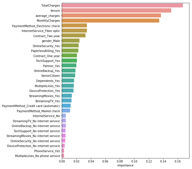
Features importances
rnd_clf = RandomForestClassifier(n_estimators=500, n_jobs=-1)
rnd_clf.fit(X, y)
RandomForestClassifier(bootstrap=True, class_weight=None, criterion='gini',
            max_depth=None, max_features='auto', max_leaf_nodes=None,
            min_impurity_decrease=0.0, min_impurity_split=None,
            min_samples_leaf=1, min_samples_split=2,
            min_weight_fraction_leaf=0.0, n_estimators=500, n_jobs=-1,
            oob_score=False, random_state=None, verbose=0,
            warm_start=False)
feature_importances = pd.DataFrame(rnd_clf.feature_importances_, index = X.columns,
                                    columns=['importance']).sort_values('importance', ascending=False)
feature_importances[:10]
| importance | |
|---|---|
| TotalCharges | 0.167416 |
| tenure | 0.150908 |
| average_charges | 0.137030 |
| MonthlyCharges | 0.134679 |
| PaymentMethod_Electronic check | 0.034640 |
| InternetService_Fiber optic | 0.034376 |
| Contract_Two year | 0.032602 |
| gender_Male | 0.024216 |
| OnlineSecurity_Yes | 0.022954 |
| PaperlessBilling_Yes | 0.022600 |
plt.figure(figsize=(8, 10))
sns.barplot(x="importance", y=feature_importances.index, data=feature_importances)
plt.show()
Baselines
# f1_score binary by default
def get_f1_scores(clf, model_name):
    y_train_pred, y_pred = clf.predict(X_train), clf.predict(X_test)
    print(model_name, f'\t - Training F1 score = {f1_score(y_train, y_train_pred) * 100:.2f}% / Test F1 score = {f1_score(y_test, y_pred)  * 100:.2f}%')
model_list = [RandomForestClassifier(),
    LogisticRegression(),
    SVC(),
    LinearSVC(),
    SGDClassifier(),
    lgbm.LGBMClassifier(),
    xgb.XGBClassifier()
             ]
model_names = [str(m)[:str(m).index('(')] for m in model_list]
for model, name in zip(model_list, model_names):
    model.fit(X_train, y_train)
    get_f1_scores(model, name)
RandomForestClassifier 	 - Training F1 score = 95.88% / Test F1 score = 51.62%
LogisticRegression 	 - Training F1 score = 60.45% / Test F1 score = 56.12%
SVC 	 - Training F1 score = 58.92% / Test F1 score = 54.46%
LinearSVC 	 - Training F1 score = 59.91% / Test F1 score = 56.36%
SGDClassifier 	 - Training F1 score = 40.85% / Test F1 score = 36.83%
LGBMClassifier 	 - Training F1 score = 76.50% / Test F1 score = 57.02%
XGBClassifier 	 - Training F1 score = 62.61% / Test F1 score = 58.36%
The 1st model - RandomForrest Clf - is clearly overfitting the train dataset and can’t generalize. The others models don’t have good results and are probably underfitting. So let’s tuned them !
Training more accurately other models
Randomforest with weighted classes
rfc = RandomForestClassifier()
rfc.fit(X_train, y_train)
get_f1_scores(rfc, 'RandomForest')
RandomForest - Training F1 score = 96.83% / Test F1 score = 48.52%
y.sum(), len(y) - y.sum()
(1869, 5163)
rfc = RandomForestClassifier(class_weight={1:1869, 0:5174})
rfc.fit(X_train, y_train)
get_f1_scores(rfc, 'RandomForest weighted')
RandomForest weighted - Training F1 score = 96.35% / Test F1 score = 51.89%
The improvement is not significant…
LGBM with weighted classes
lgbm_w = lgbm.LGBMClassifier(n_jobs = -1, class_weight={0:1869, 1:5174})
lgbm_w.fit(X_train, y_train)
get_f1_scores(lgbm_w, 'LGBM weighted')
LGBM weighted - Training F1 score = 78.76% / Test F1 score = 63.03%
XGB with ratio
ratio = ((len(y) - y.sum()) - y.sum()) / y.sum()
ratio
1.7624398073836276
xgb_model = xgb.XGBClassifier(objective="binary:logistic", scale_pos_weight=ratio)
xgb_model.fit(X_train, y_train)
get_f1_scores(xgb_model, 'XGB with ratio')
XGB with ratio - Training F1 score = 66.48% / Test F1 score = 63.47%
That’s a little better.
Adaboost
abc = AdaBoostClassifier()
abc.fit(X_train, y_train)
get_f1_scores(abc, 'Adaboost')
Adaboost - Training F1 score = 60.75% / Test F1 score = 58.05%
Using GridsearchCV & Combining the best models
With XGB
print(classification_report(y_test, xgb_model.predict(X_test)))
              precision    recall  f1-score   support

           0       0.87      0.81      0.84      1018
           1       0.58      0.70      0.63       389

   micro avg       0.78      0.78      0.78      1407
   macro avg       0.73      0.75      0.74      1407
weighted avg       0.79      0.78      0.78      1407
Let’s use a GridSearch with 5 cross validation to tuned the hyperparameters
from sklearn.model_selection import GridSearchCV
params = {'learning_rate':[0.175, 0.167, 0.165, 0.163, 0.17],
          'max_depth':[1, 2, 3],
          'scale_pos_weight':[1.70, 1.73, 1.76, 1.79]}
clf_grid = GridSearchCV(xgb.XGBClassifier(), param_grid=params, cv=5, scoring='f1', n_jobs=-1, verbose=1)
clf_grid.fit(X_train, y_train)
Fitting 5 folds for each of 60 candidates, totalling 300 fits


[Parallel(n_jobs=-1)]: Using backend LokyBackend with 8 concurrent workers.
[Parallel(n_jobs=-1)]: Done  34 tasks      | elapsed:    2.6s
[Parallel(n_jobs=-1)]: Done 184 tasks      | elapsed:   10.3s
[Parallel(n_jobs=-1)]: Done 300 out of 300 | elapsed:   16.2s finished


GridSearchCV(cv=5, error_score='raise-deprecating',
       estimator=XGBClassifier(base_score=0.5, booster='gbtree', colsample_bylevel=1,
       colsample_bytree=1, gamma=0, learning_rate=0.1, max_delta_step=0,
       max_depth=3, min_child_weight=1, missing=None, n_estimators=100,
       n_jobs=1, nthread=None, objective='binary:logistic', random_state=0,
       reg_alpha=0, reg_lambda=1, scale_pos_weight=1, seed=None,
       silent=True, subsample=1),
       fit_params=None, iid='warn', n_jobs=-1,
       param_grid={'learning_rate': [0.175, 0.167, 0.165, 0.163, 0.17], 'max_depth': [1, 2, 3], 'scale_pos_weight': [1.7, 1.73, 1.76, 1.79]},
       pre_dispatch='2*n_jobs', refit=True, return_train_score='warn',
       scoring='f1', verbose=1)
clf_grid.best_score_
0.635398553168061
clf_grid.best_params_
{'learning_rate': 0.163, 'max_depth': 1, 'scale_pos_weight': 1.76}
With a LogisticRegression
lr = LogisticRegression(C=10, class_weight={0:0.26, 1:0.74})
lr.fit(X_train, y_train)
get_f1_scores(lr, 'Logistic Reg')
Logistic Reg - Training F1 score = 62.82% / Test F1 score = 64.88%
Now we can try to combine the best models
xgb_model = xgb.XGBClassifier(objective="binary:logistic", learning_rate=0.167, max_depth=2, scale_pos_weight=1.73)
xgb_model.fit(X_train, y_train)
get_f1_scores(xgb_model, 'XGB with ratio')
XGB with ratio - Training F1 score = 66.17% / Test F1 score = 63.93%
y_pred_lr = lr.predict_proba(X_test)
lgbm_w = lgbm.LGBMClassifier(n_jobs = -1, class_weight={0:1869, 1:5174})
lgbm_w.fit(X_train, y_train)
y_pred_lgbm = lgbm_w.predict_proba(X_test)
# y_pred with predict_proba returns 2 cols, one for each class
y_pred_xgb = xgb_model.predict_proba(X_test)
y_pred_xgb[:5, 1]
array([0.66343373, 0.6869538 , 0.031379  , 0.49967214, 0.06845096],
      dtype=float32)
y_pred_lgbm[:5, 1]
array([0.65824753, 0.73075217, 0.06651954, 0.50086417, 0.0424213 ])
test = np.vstack((y_pred_lgbm[:5, 1], y_pred_xgb[:5, 1]))
test
array([[0.65824753, 0.73075217, 0.06651954, 0.50086417, 0.0424213 ],
       [0.66343373, 0.68695378, 0.031379  , 0.49967214, 0.06845096]])
np.mean(test, axis=0)
array([0.66084063, 0.70885298, 0.04894927, 0.50026816, 0.05543613])
y_pred_mean = np.mean(np.vstack((y_pred_lgbm[:, 1], y_pred_xgb[:, 1])), axis=0)
y_pred_mean[:5]
array([0.66084063, 0.70885298, 0.04894927, 0.50026816, 0.05543613])
y_pred_mean[y_pred_mean < 0.5] = 0
y_pred_mean[y_pred_mean > 0.5] = 1
y_pred_mean[:5]
array([1., 1., 0., 1., 0.])
print(f'F1 score of models combined on the test dataset = {f1_score(y_test, y_pred_mean) * 100:.2f}%')
F1 score of models combined on the test dataset = 63.59%
Despite combining model, the best F1 score is still obtained by XGB with tuned hyperparameters.
