
Analysis of the Car Datasheet
import warnings
warnings.simplefilter(action='ignore', category=FutureWarning)

import pandas as pd

%matplotlib inline
import matplotlib.pyplot as plt
import seaborn as sns

SCRAPED_CSV = 'scraped_cars.csv'
Load CSV and Review
df_raw = pd.read_csv(SCRAPED_CSV)
df = df_raw.copy() # keep a defensive copy of the original data
df.tail()
| name | cylinders | weight | year | territory | acceleration | mpg | hp | displacement | |
|---|---|---|---|---|---|---|---|---|---|
| 401 | Ford Mustang Gl | 4 | 2790 | 1982 | USA | 15.6 | 27.0 | 86.0 | 140.0 |
| 402 | Vw Pickup | 4 | 2130 | 1982 | Europe | 24.6 | 44.0 | 52.0 | 97.0 |
| 403 | Dodge Rampage | 4 | 2295 | 1982 | USA | 11.6 | 32.0 | 84.0 | 135.0 |
| 404 | Ford Ranger | 4 | 2625 | 1982 | USA | 18.6 | 28.0 | 79.0 | 120.0 |
| 405 | Chevy S-10 | 4 | 2720 | 1982 | USA | 19.4 | 31.0 | 82.0 | 119.0 |
df.shape
(406, 9)
df.sample(5)
| name | cylinders | weight | year | territory | acceleration | mpg | hp | displacement | |
|---|---|---|---|---|---|---|---|---|---|
| 54 | Pontiac Firebird | 6 | 3282 | 1971 | USA | 15.0 | 19.0 | 100.0 | 250.0 |
| 313 | Chevrolet Citation | 6 | 2595 | 1979 | USA | 11.3 | 28.8 | 115.0 | 173.0 |
| 175 | Ford Pinto | 4 | 2639 | 1975 | USA | 17.0 | 23.0 | 83.0 | 140.0 |
| 75 | Buick Lesabre Custom | 8 | 4502 | 1972 | USA | 13.5 | 13.0 | 155.0 | 350.0 |
| 110 | Chevrolet Impala | 8 | 4997 | 1973 | USA | 14.0 | 11.0 | 150.0 | 400.0 |
df.describe()
| cylinders | weight | year | acceleration | mpg | hp | displacement | |
|---|---|---|---|---|---|---|---|
| count | 406.000000 | 406.000000 | 406.000000 | 406.000000 | 398.000000 | 400.000000 | 406.000000 |
| mean | 5.475369 | 2979.413793 | 1975.921182 | 15.519704 | 23.514573 | 105.082500 | 194.779557 |
| std | 1.712160 | 847.004328 | 3.748737 | 2.803359 | 7.815984 | 38.768779 | 104.922458 |
| min | 3.000000 | 1613.000000 | 1970.000000 | 8.000000 | 9.000000 | 46.000000 | 68.000000 |
| 25% | 4.000000 | 2226.500000 | 1973.000000 | 13.700000 | 17.500000 | 75.750000 | 105.000000 |
| 50% | 4.000000 | 2822.500000 | 1976.000000 | 15.500000 | 23.000000 | 95.000000 | 151.000000 |
| 75% | 8.000000 | 3618.250000 | 1979.000000 | 17.175000 | 29.000000 | 130.000000 | 302.000000 |
| max | 8.000000 | 5140.000000 | 1982.000000 | 24.800000 | 46.600000 | 230.000000 | 455.000000 |
Data Review Strategy
df.territory.value_counts()
USA       254
Japan      79
Europe     73
Name: territory, dtype: int64
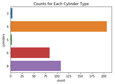
df.cylinders.value_counts()
4    207
8    108
6     84
3      4
5      3
Name: cylinders, dtype: int64
df.cylinders.value_counts().sort_index()
3      4
4    207
5      3
6     84
8    108
Name: cylinders, dtype: int64
ax = sns.countplot(data=df, y='cylinders')
ax.set_title("Counts for Each Cylinder Type");
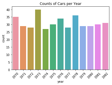
ax = sns.countplot(data=df, x='year')
ax.set_title('Counts of Cars per Year');
plt.xticks(rotation=45);
df.isnull().sum()
name            0
cylinders       0
weight          0
year            0
territory       0
acceleration    0
mpg             8
hp              6
displacement    0
dtype: int64
df.mpg.isnull()[5:15]
5     False
6     False
7     False
8     False
9     False
10     True
11     True
12     True
13     True
14     True
Name: mpg, dtype: bool
df[df.mpg.isnull()]
| name | cylinders | weight | year | territory | acceleration | mpg | hp | displacement | |
|---|---|---|---|---|---|---|---|---|---|
| 10 | Citroen Ds-21 Pallas | 4 | 3090 | 1970 | Europe | 17.5 | NaN | 115.0 | 133.0 |
| 11 | Chevrolet Chevelle Concours (Sw) | 8 | 4142 | 1970 | USA | 11.5 | NaN | 165.0 | 350.0 |
| 12 | Ford Torino (Sw) | 8 | 4034 | 1970 | USA | 11.0 | NaN | 153.0 | 351.0 |
| 13 | Plymouth Satellite (Sw) | 8 | 4166 | 1970 | USA | 10.5 | NaN | 175.0 | 383.0 |
| 14 | Amc Rebel Sst (Sw) | 8 | 3850 | 1970 | USA | 11.0 | NaN | 175.0 | 360.0 |
| 17 | Ford Mustang Boss 302 | 8 | 3353 | 1970 | USA | 8.0 | NaN | 140.0 | 302.0 |
| 39 | Volkswagen Super Beetle 117 | 4 | 1978 | 1971 | Europe | 20.0 | NaN | 48.0 | 97.0 |
| 367 | Saab 900S | 4 | 2800 | 1981 | Europe | 15.4 | NaN | 110.0 | 121.0 |
df[df.hp.isnull()]
| name | cylinders | weight | year | territory | acceleration | mpg | hp | displacement | |
|---|---|---|---|---|---|---|---|---|---|
| 38 | Ford Pinto | 4 | 2046 | 1971 | USA | 19.0 | 25.0 | NaN | 98.0 |
| 133 | Ford Maverick | 6 | 2875 | 1974 | USA | 17.0 | 21.0 | NaN | 200.0 |
| 337 | Renault Lecar Deluxe | 4 | 1835 | 1980 | Europe | 17.3 | 40.9 | NaN | 85.0 |
| 343 | Ford Mustang Cobra | 4 | 2905 | 1980 | USA | 14.3 | 23.6 | NaN | 140.0 |
| 361 | Renault 18I | 4 | 2320 | 1981 | Europe | 15.8 | 34.5 | NaN | 100.0 |
| 382 | Amc Concord Dl | 4 | 3035 | 1982 | USA | 20.5 | 23.0 | NaN | 151.0 |
def highlight_max(s):
    '''Highlight the maximum in a Series yellow'''
    is_max = s == s.max()
    return ['background-color: yellow' if v else '' for v in is_max]

df.pivot_table(index=['year'], aggfunc='count').style.apply(highlight_max, axis=1)
| acceleration | cylinders | displacement | hp | mpg | name | territory | weight | |
|---|---|---|---|---|---|---|---|---|
| year | ||||||||
| 1970 | 35 | 35 | 35 | 35 | 29 | 35 | 35 | 35 |
| 1971 | 29 | 29 | 29 | 28 | 28 | 29 | 29 | 29 |
| 1972 | 28 | 28 | 28 | 28 | 28 | 28 | 28 | 28 |
| 1973 | 40 | 40 | 40 | 40 | 40 | 40 | 40 | 40 |
| 1974 | 27 | 27 | 27 | 26 | 27 | 27 | 27 | 27 |
| 1975 | 30 | 30 | 30 | 30 | 30 | 30 | 30 | 30 |
| 1976 | 34 | 34 | 34 | 34 | 34 | 34 | 34 | 34 |
| 1977 | 28 | 28 | 28 | 28 | 28 | 28 | 28 | 28 |
| 1978 | 36 | 36 | 36 | 36 | 36 | 36 | 36 | 36 |
| 1979 | 29 | 29 | 29 | 29 | 29 | 29 | 29 | 29 |
| 1980 | 29 | 29 | 29 | 27 | 29 | 29 | 29 | 29 |
| 1981 | 30 | 30 | 30 | 29 | 29 | 30 | 30 | 30 |
| 1982 | 31 | 31 | 31 | 30 | 31 | 31 | 31 | 31 |
print(f"Before we drop NaN rows we have {df.shape} rows")
df = df.dropna()
print(f"After we drop NaN rows we have {df.shape} rows")
Before we drop NaN rows we have (406, 9) rows
After we drop NaN rows we have (392, 9) rows
df.cylinders.value_counts().sort_index()
3      4
4    199
5      3
6     83
8    103
Name: cylinders, dtype: int64
df = df.query("cylinders != 3 and cylinders != 5").copy()
df.cylinders.value_counts().sort_index()
4    199
6     83
8    103
Name: cylinders, dtype: int64
df['cylinders_label'] = df.cylinders.apply(lambda v: f"{v} cylinders")
df.cylinders_label.value_counts().sort_index()
4 cylinders    199
6 cylinders     83
8 cylinders    103
Name: cylinders_label, dtype: int64
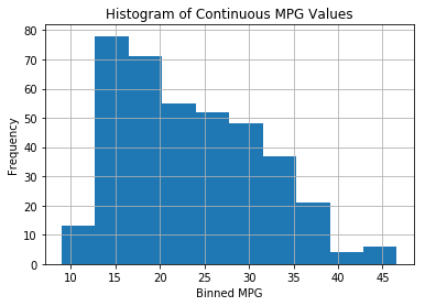
What Distribution Does MPG Have?
print(f"Examples of MPG values: {list(df.mpg.sample(10).sort_values())}")
ax = df.mpg.hist()
ax.set_ylabel('Frequency')
ax.set_xlabel('Binned MPG')
ax.set_title('Histogram of Continuous MPG Values');
Examples of MPG values: [14.0, 17.0, 18.0, 20.2, 23.5, 24.0, 25.0, 30.5, 36.0, 37.2]
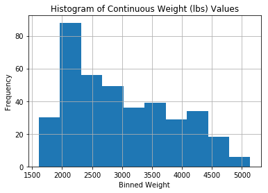
ax = df.weight.hist()
ax.set_ylabel('Frequency')
ax.set_xlabel('Binned Weight')
ax.set_title('Histogram of Continuous Weight (lbs) Values');
Reviewing Our Goal
df.pivot_table(index=['year'], aggfunc='mean')
| acceleration | cylinders | displacement | hp | mpg | weight | |
|---|---|---|---|---|---|---|
| year | ||||||
| 1970 | 12.948276 | 6.758621 | 281.413793 | 147.827586 | 17.689655 | 3372.793103 |
| 1971 | 15.000000 | 5.629630 | 213.888889 | 107.037037 | 21.111111 | 3030.592593 |
| 1972 | 15.185185 | 5.925926 | 223.870370 | 121.037037 | 18.703704 | 3271.333333 |
| 1973 | 14.333333 | 6.461538 | 261.666667 | 131.512821 | 17.076923 | 3452.230769 |
| 1974 | 16.173077 | 5.230769 | 170.653846 | 94.230769 | 22.769231 | 2878.038462 |
| 1975 | 16.050000 | 5.600000 | 205.533333 | 101.066667 | 20.266667 | 3176.800000 |
| 1976 | 15.941176 | 5.647059 | 197.794118 | 101.117647 | 21.573529 | 3078.735294 |
| 1977 | 15.507407 | 5.555556 | 195.518519 | 104.888889 | 23.444444 | 3007.629630 |
| 1978 | 15.802857 | 5.371429 | 179.142857 | 99.600000 | 24.168571 | 2862.714286 |
| 1979 | 15.660714 | 5.857143 | 207.535714 | 102.071429 | 25.082143 | 3038.392857 |
| 1980 | 17.084000 | 4.160000 | 117.720000 | 77.000000 | 34.104000 | 2422.120000 |
| 1981 | 16.325000 | 4.642857 | 136.571429 | 81.035714 | 30.185714 | 2530.178571 |
| 1982 | 16.510000 | 4.200000 | 128.133333 | 81.466667 | 32.000000 | 2434.166667 |
What Correlates with MPG?
df.corr()['mpg'].sort_values()
weight         -0.842681
displacement   -0.817887
cylinders      -0.794872
hp             -0.780259
acceleration    0.419337
year            0.579778
mpg             1.000000
Name: mpg, dtype: float64
Exploring MPG vs. Weight
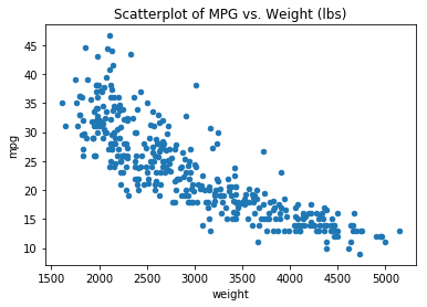
ax = df.plot(kind="scatter", x='weight', y='mpg')
ax.set_title('Scatterplot of MPG vs. Weight (lbs)');
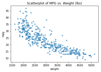
ax = df.plot(kind="scatter", x='weight', y='mpg', alpha=0.5)
ax.set_title('Scatterplot of MPG vs. Weight (lbs)');
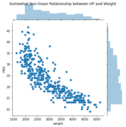
jg = sns.jointplot(data=df, x='weight', y='mpg');
jg.fig.suptitle('Somewhat Non-linear Relationship between HP and Weight');
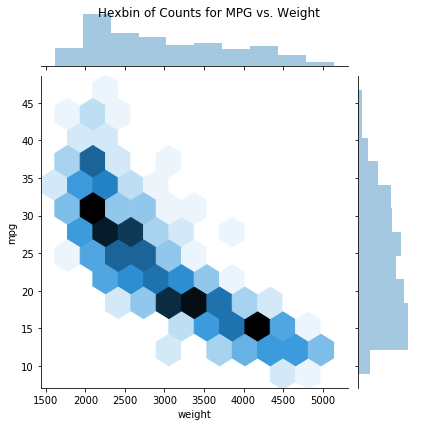
jg=sns.jointplot(data=df, x='weight', y='mpg', kind='hexbin')
jg.fig.suptitle('Hexbin of Counts for MPG vs. Weight');
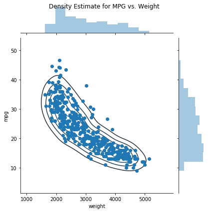
jg = sns.jointplot(data=df, x='weight', y='mpg').plot_joint(sns.kdeplot, zorder=0, n_levels=5)
jg.fig.suptitle('Density Estimate for MPG vs. Weight');
Exploring HP vs. Weight
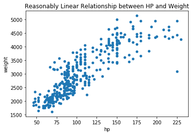
ax = df.plot(kind="scatter", x='hp', y='weight')
ax.set_title('Reasonably Linear Relationship between HP and Weight');
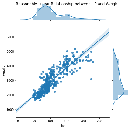
jg = sns.jointplot(data=df, x='hp', y='weight', kind='reg')
jg.fig.suptitle('Reasonably Linear Relationship between HP and Weight');
df.query("hp > 200 and weight < 3500") # Fully equipped luxury entrant
| name | cylinders | weight | year | territory | acceleration | mpg | hp | displacement | cylinders_label | |
|---|---|---|---|---|---|---|---|---|---|---|
| 19 | Buick Estate Wagon (Sw) | 8 | 3086 | 1970 | USA | 10.0 | 14.0 | 225.0 | 455.0 | 8 cylinders |
Cylinders and Displacement
sorted_cylinders_label = df.cylinders_label.value_counts().sort_index().index
sorted_cylinders_label
Index(['4 cylinders', '6 cylinders', '8 cylinders'], dtype='object')
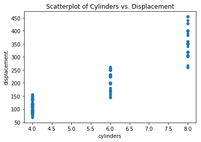
ax = df.plot(kind='scatter', x='cylinders', y='displacement')
ax.set_title("Scatterplot of Cylinders vs. Displacement");
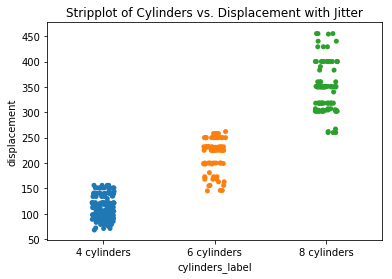
ax = sns.stripplot(data=df, x='cylinders_label', y='displacement', order=sorted_cylinders_label)
ax.set_title("Stripplot of Cylinders vs. Displacement with Jitter");
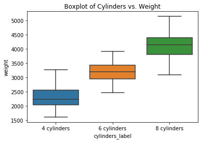
ax = sns.boxplot(data=df, x='cylinders_label', y='weight', order=sorted_cylinders_label)
ax.set_title("Boxplot of Cylinders vs. Weight");
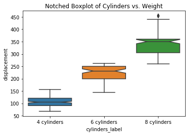
ax = sns.boxplot(data=df, x='cylinders_label', y='displacement', order=sorted_cylinders_label, notch=True)
ax.set_title("Notched Boxplot of Cylinders vs. Weight");
Looking at MPG over Time
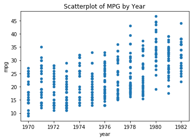
ax = df.plot(kind="scatter", x='year', y='mpg');
ax.set_title('Scatterplot of MPG by Year');
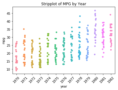
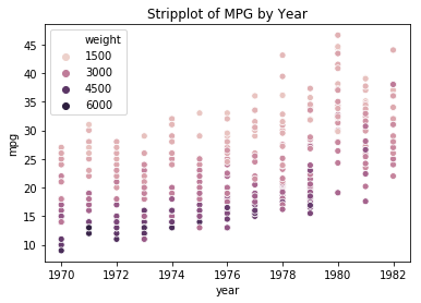
ax = sns.stripplot(data=df, x='year', y='mpg')
ax.set_title('Stripplot of MPG by Year');
plt.xticks(rotation=45);
ax = sns.boxplot(data=df, x='year', y='mpg')
ax.set_title("Boxplot of MPG by Year");
plt.xticks(rotation=45);
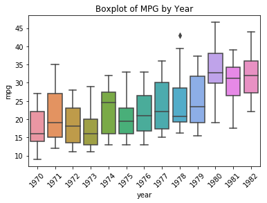
df.query('year=="1978" and mpg > 40')
| name | cylinders | weight | year | territory | acceleration | mpg | hp | displacement | cylinders_label | |
|---|---|---|---|---|---|---|---|---|---|---|
| 251 | Volkswagen Rabbit Custom Diesel | 4 | 1985 | 1978 | Europe | 21.5 | 43.1 | 48.0 | 90.0 | 4 cylinders |
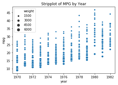
ax = sns.scatterplot(data=df, x='year', y='mpg', size='weight')
ax.set_title('Stripplot of MPG by Year');
ax = sns.scatterplot(data=df, x='year', y='mpg', hue='weight')
ax.set_title('Stripplot of MPG by Year');
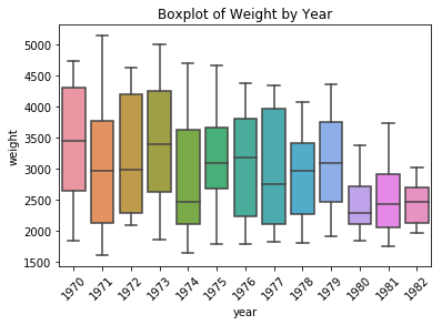
ax = sns.boxplot(data=df, x='year', y='weight')
ax.set_title('Boxplot of Weight by Year');
plt.xticks(rotation=45);
Text analysis
df.head()
| name | cylinders | weight | year | territory | acceleration | mpg | hp | displacement | cylinders_label | |
|---|---|---|---|---|---|---|---|---|---|---|
| 0 | Chevrolet Chevelle Malibu | 8 | 3504 | 1970 | USA | 12.0 | 18.0 | 130.0 | 307.0 | 8 cylinders |
| 1 | Buick Skylark 320 | 8 | 3693 | 1970 | USA | 11.5 | 15.0 | 165.0 | 350.0 | 8 cylinders |
| 2 | Plymouth Satellite | 8 | 3436 | 1970 | USA | 11.0 | 18.0 | 150.0 | 318.0 | 8 cylinders |
| 3 | Amc Rebel Sst | 8 | 3433 | 1970 | USA | 12.0 | 16.0 | 150.0 | 304.0 | 8 cylinders |
| 4 | Ford Torino | 8 | 3449 | 1970 | USA | 10.5 | 17.0 | 140.0 | 302.0 | 8 cylinders |
ser_car_makes = df.name.str.lower().str.split(n=1, expand=True)[0]
ser_car_makes.value_counts()[:10]
ford          48
chevrolet     43
plymouth      31
dodge         28
amc           27
toyota        25
datsun        23
buick         17
pontiac       16
volkswagen    15
Name: 0, dtype: int64
ser_car_makes.value_counts()[-10:]
mercedes-benz    2
cadillac         2
toyouta          1
triumph          1
maxda            1
chevroelt        1
capri            1
vokswagen        1
nissan           1
hi               1
Name: 0, dtype: int64
df['car_makes'] = ser_car_makes
ser_cars_by_territory = df[['territory', 'car_makes']].pivot_table(index=['territory', 'car_makes'], aggfunc='size')
df_cars_by_territory = pd.DataFrame(ser_cars_by_territory) # anonymous Series
df_cars_by_territory.columns = ['size'] # rename anonymous column 0 to a named column
df_cars_by_territory = df_cars_by_territory.sort_values(by=['territory', 'size'], ascending=False)
df_cars_by_territory
| size | ||
|---|---|---|
| territory | car_makes | |
| USA | ford | 48 |
| chevrolet | 43 | |
| plymouth | 31 | |
| dodge | 28 | |
| amc | 27 | |
| buick | 17 | |
| pontiac | 16 | |
| mercury | 11 | |
| oldsmobile | 10 | |
| chrysler | 6 | |
| chevy | 3 | |
| cadillac | 2 | |
| capri | 1 | |
| chevroelt | 1 | |
| hi | 1 | |
| Japan | toyota | 25 |
| datsun | 23 | |
| honda | 13 | |
| mazda | 7 | |
| subaru | 4 | |
| maxda | 1 | |
| nissan | 1 | |
| toyouta | 1 | |
| Europe | volkswagen | 15 |
| fiat | 8 | |
| peugeot | 8 | |
| volvo | 6 | |
| vw | 6 | |
| audi | 5 | |
| opel | 4 | |
| saab | 4 | |
| renault | 3 | |
| bmw | 2 | |
| mercedes-benz | 2 | |
| triumph | 1 | |
| vokswagen | 1 |
mask = df_cars_by_territory.apply(lambda x: x['size'] > 10, axis=1)
df_cars_by_territory[mask]
| size | ||
|---|---|---|
| territory | car_makes | |
| USA | ford | 48 |
| chevrolet | 43 | |
| plymouth | 31 | |
| dodge | 28 | |
| amc | 27 | |
| buick | 17 | |
| pontiac | 16 | |
| mercury | 11 | |
| Japan | toyota | 25 |
| datsun | 23 | |
| honda | 13 | |
| Europe | volkswagen | 15 |
Report
This report answers the following questions:
- Is there a relationship between Weight and MPG - yes, with more weight we generally see lower MPG
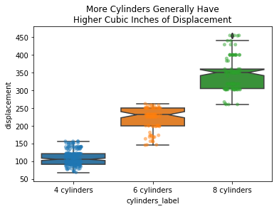
- Is there a relationship between Cylinders and Displacement - yes, with more Cylinders we see a higher Displacement
- Is there a relationship between MPG and Years - yes, generally as we move from 1970 to 1982 we see steady improvements in MPG
print(f"df_raw had shape {df_raw.shape}, after dropping NaN entries we \
reduced from {df_raw.shape[0]} to {df.shape[0]} rows.")

assert ((df.mpg >= 7) & (df.mpg <=47)).all(), "Why do we see a wider range of MPG values now?"
assert ((df.year >= 1970) & (df.year <= 1982)).all(), "Why do we see a wider range of years now?"
df_raw had shape (406, 9), after dropping NaN entries we reduced from 406 to 385 rows.
As weight increases we see a decrease in MPG, this relationship is slightly non-linear with a faster decrease in MPG associated with low-to-mid Weight.
jg = sns.jointplot(data=df, x='weight', y='mpg').plot_joint(sns.kdeplot, zorder=0, n_levels=5)
jg.fig.suptitle('Density Estimate for MPG vs. Weight');

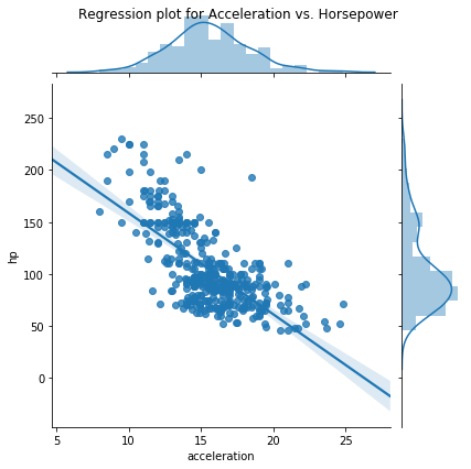
Acceleration gets worse as Horsepower decreases.
jg = sns.jointplot(data=df, x='acceleration', y='hp', kind='reg')
jg.fig.suptitle('Regression plot for Acceleration vs. Horsepower');
An engine’s cubic inches of displacement is strongly related to the count of Cylinders.
ax = sns.boxplot(data=df, x='cylinders_label', y='displacement', order=sorted_cylinders_label, notch=True)
sns.stripplot(data=df, x='cylinders_label', y='displacement', order=sorted_cylinders_label, alpha=0.5, ax=ax)
ax.set_title("More Cylinders Generally Have\nHigher Cubic Inches of Displacement");
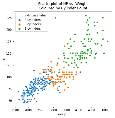
Heavier vehicles tend to have more Horsepower, the heaviest vehicles have the highest count of Cylinders.
fig, ax = plt.subplots(figsize=(6, 6))
sns.scatterplot(data=df, x='weight', y='hp', hue='cylinders_label',
                     hue_order=sorted_cylinders_label, ax=ax)
ax.set_title('Scatterplot of HP vs. Weight\nColoured by Cylinder Count');
Vehicle brands are strongly associated with Territory.
cm = sns.light_palette("green", as_cmap=True)
mask = df_cars_by_territory.apply(lambda x: x['size'] > 10, axis=1)
df_cars_by_territory[mask].style.background_gradient(cmap=cm)
| size | ||
|---|---|---|
| territory | car_makes | |
| USA | ford | 48 |
| chevrolet | 43 | |
| plymouth | 31 | |
| dodge | 28 | |
| amc | 27 | |
| buick | 17 | |
| pontiac | 16 | |
| mercury | 11 | |
| Japan | toyota | 25 |
| datsun | 23 | |
| honda | 13 | |
| Europe | volkswagen | 15 |
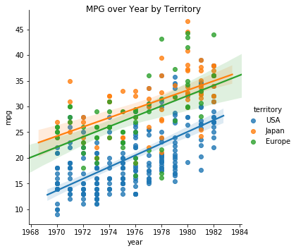
Vehicles from the USA consistently have worse MPG than corresponding vehicles from Japan or Europe in this sample. Vehicles in each territory become more efficient over the Years.
fg = sns.lmplot(data=df, x='year', y='mpg', hue='territory')
fg.fig.suptitle('MPG over Year by Territory');