

Quora Insincere Questions Classification - Part 1/2
Side note : this is the first part of two, see the conclusion for the next part.
Context
An existential problem for any major website today is how to handle toxic and divisive content. Quora wants to tackle this problem head-on to keep their platform a place where users can feel safe sharing their knowledge with the world.
Quora is a platform that empowers people to learn from each other. On Quora, people can ask questions and connect with others who contribute unique insights and quality answers. A key challenge is to weed out insincere questions – those founded upon false premises, or that intend to make a statement rather than look for helpful answers.
In this competition, Kagglers will develop models that identify and flag insincere questions. To date, Quora has employed both machine learning and manual review to address this problem. With your help, they can develop more scalable methods to detect toxic and misleading content.
Here’s your chance to combat online trolls at scale. Help Quora uphold their policy of “Be Nice, Be Respectful” and continue to be a place for sharing and growing the world’s knowledge.
Goal
Predict whether a question asked on Quora is sincere or not
An insincere question is defined as a question intended to make a statement rather than look for helpful answers. Some characteristics that can signify that a question is insincere:
- Has a non-neutral tone
- Is disparaging or inflammatory
- Isn’t grounded in reality
- Uses sexual content (incest, bestiality, pedophilia) for shock value, and not to seek genuine answers
Dataset
The training data includes the question that was asked, and whether it was identified as insincere (target = 1). The ground-truth labels contain some amount of noise: they are not guaranteed to be perfect.
Note that the distribution of questions in the dataset should not be taken to be representative of the distribution of questions asked on Quora. This is, in part, because of the combination of sampling procedures and sanitization measures that have been applied to the final dataset.
Exploratory Data Analysis
Libraries import
import warnings
warnings.filterwarnings("ignore")
import numpy as np
import pandas as pd

import seaborn as sns
import matplotlib.pyplot as plt
%matplotlib inline
from nltk.tokenize import word_tokenize
from nltk.corpus import stopwords
from nltk.stem import PorterStemmer

from string import punctuation

from sklearn.model_selection import train_test_split
from sklearn.pipeline import Pipeline
from sklearn.linear_model import LogisticRegression
from sklearn.feature_extraction.text import CountVectorizer, TfidfVectorizer
from sklearn.metrics import f1_score, classification_report
from xgboost import XGBClassifier
import lightgbm as lgb
File descriptions
- train.csv - the training set
- test.csv - the test set
- sample_submission.csv - A sample submission in the correct format
- enbeddings/ - (see below)
df = pd.read_csv("../input/quora-insincere-questions-classification/train.csv")
df.head()
| qid | question_text | target | |
|---|---|---|---|
| 0 | 00002165364db923c7e6 | How did Quebec nationalists see their province... | 0 |
| 1 | 000032939017120e6e44 | Do you have an adopted dog, how would you enco... | 0 |
| 2 | 0000412ca6e4628ce2cf | Why does velocity affect time? Does velocity a... | 0 |
| 3 | 000042bf85aa498cd78e | How did Otto von Guericke used the Magdeburg h... | 0 |
| 4 | 0000455dfa3e01eae3af | Can I convert montra helicon D to a mountain b... | 0 |
Data fields
- qid - unique question identifier
- question_text - Quora question text
- target - a question labeled “insincere” has a value of 1, otherwise 0
pd.read_csv("../input/quora-insincere-questions-classification/test.csv").head()
| qid | question_text | |
|---|---|---|
| 0 | 0000163e3ea7c7a74cd7 | Why do so many women become so rude and arroga... |
| 1 | 00002bd4fb5d505b9161 | When should I apply for RV college of engineer... |
| 2 | 00007756b4a147d2b0b3 | What is it really like to be a nurse practitio... |
| 3 | 000086e4b7e1c7146103 | Who are entrepreneurs? |
| 4 | 0000c4c3fbe8785a3090 | Is education really making good people nowadays? |
Basic infos and analysis of the target
df.info()
<class 'pandas.core.frame.DataFrame'>
RangeIndex: 1306122 entries, 0 to 1306121
Data columns (total 3 columns):
qid              1306122 non-null object
question_text    1306122 non-null object
target           1306122 non-null int64
dtypes: int64(1), object(2)
memory usage: 29.9+ MB
No Nan and no duplicated line :
df.duplicated().sum()
0
Target analysis
df.target.value_counts()
0    1225312
1      80810
Name: target, dtype: int64
df.target.describe()
count    1.306122e+06
mean     6.187018e-02
std      2.409197e-01
min      0.000000e+00
25%      0.000000e+00
50%      0.000000e+00
75%      0.000000e+00
max      1.000000e+00
Name: target, dtype: float64
plt.figure(figsize=(5, 4))
sns.countplot(x='target', data=df)
plt.title('Reparition of question by sincerity (insincere = 1)');
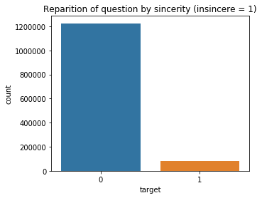
print(f'There are {df.target.sum() / df.shape[0] * 100 :.1f}% of insincere questions, which make the dataset highly unbalanced.')
There are 6.2% of insincere questions, which make the dataset highly unbalanced.
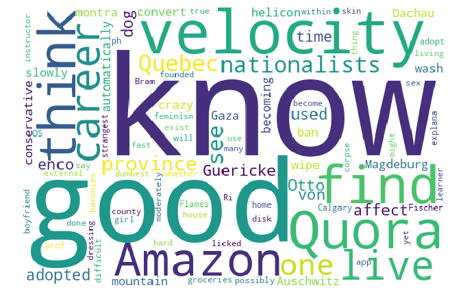
Word clouds
Generally, though, data scientists don’t think much of word clouds, in large part because the placement of the words doesn’t mean anything other than “here’s some space where I was able to fit a word.” Anyway, clouds can come handy to have a frist insight of the most common words…
Word clouds (also known as text clouds or tag clouds) work in a simple way: the more a specific word appears in a source of textual data (such as a speech, blog post, or database), the bigger and bolder it appears in the word cloud.
from wordcloud import WordCloud, STOPWORDS
stopwords = set(STOPWORDS)
print('Word cloud image generated from sincere questions')
sincere_wordcloud = WordCloud(width=600, height=400, background_color ='white', min_font_size = 10).generate(str(df[df["target"] == 0]["question_text"]))
#Positive Word cloud
plt.figure(figsize=(15,6), facecolor=None)
plt.imshow(sincere_wordcloud)
plt.axis("off")
plt.tight_layout(pad=0)
plt.show();
Word cloud image generated from sincere questions
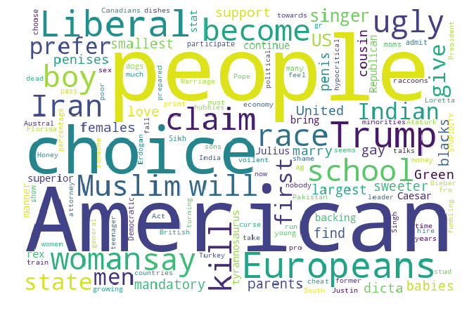
print('Word cloud image generated from INsincere questions')
insincere_wordcloud = WordCloud(width=600, height=400, background_color ='white', min_font_size = 10).generate(str(df[df["target"] == 1]["question_text"]))
#Positive Word cloud
plt.figure(figsize=(15,6), facecolor=None)
plt.imshow(insincere_wordcloud)
plt.axis("off")
plt.tight_layout(pad=0)
plt.show();
Word cloud image generated from INsincere questions
Statistics form the question texts
The process of converting data to something a computer can understand is referred to as pre-processing. One of the major forms of pre-processing is to filter out useless data. In natural language processing, useless words (data), are referred to as stop words.
# if needed
# nltk.download('stopwords')
Stop Words: A stop word is a commonly used word (such as “the”, “a”, “an”, “in”) that a search engine has been programmed to ignore, both when indexing entries for searching and when retrieving them as the result of a search query.
We would not want these words taking up space in our database, or taking up valuable processing time. For this, we can remove them easily, by storing a list of words that you consider to be stop words. NLTK(Natural Language Toolkit) in python has a list of stopwords stored in 16 different languages. You can find them in the nltk_data directory.
import nltk
from nltk.corpus import stopwords
stop_words = set(stopwords.words('english'))
stop_words
{'a',
 'about',
 'above',
 'after',
 'again',
 'against',
 'ain',
 'all',
 'am',
 'an',
 'and',
 'any',
 'are',
 'aren',
 "aren't",
 'as',
 'at',
 'be',
 'because',
 'been',
 'before',
 'being',
 'below',
 'between',
 'both',
 'but',
 'by',
 'can',
 'couldn',
 "couldn't",
 'd',
 'did',
 'didn',
 "didn't",
 'do',
 'does',
 'doesn',
 "doesn't",
 'doing',
 'don',
 "don't",
 'down',
 'during',
 'each',
 'few',
 'for',
 'from',
 'further',
 'had',
 'hadn',
 "hadn't",
 'has',
 'hasn',
 "hasn't",
 'have',
 'haven',
 "haven't",
 'having',
 'he',
 'her',
 'here',
 'hers',
 'herself',
 'him',
 'himself',
 'his',
 'how',
 'i',
 'if',
 'in',
 'into',
 'is',
 'isn',
 "isn't",
 'it',
 "it's",
 'its',
 'itself',
 'just',
 'll',
 'm',
 'ma',
 'me',
 'mightn',
 "mightn't",
 'more',
 'most',
 'mustn',
 "mustn't",
 'my',
 'myself',
 'needn',
 "needn't",
 'no',
 'nor',
 'not',
 'now',
 'o',
 'of',
 'off',
 'on',
 'once',
 'only',
 'or',
 'other',
 'our',
 'ours',
 'ourselves',
 'out',
 'over',
 'own',
 're',
 's',
 'same',
 'shan',
 "shan't",
 'she',
 "she's",
 'should',
 "should've",
 'shouldn',
 "shouldn't",
 'so',
 'some',
 'such',
 't',
 'than',
 'that',
 "that'll",
 'the',
 'their',
 'theirs',
 'them',
 'themselves',
 'then',
 'there',
 'these',
 'they',
 'this',
 'those',
 'through',
 'to',
 'too',
 'under',
 'until',
 'up',
 've',
 'very',
 'was',
 'wasn',
 "wasn't",
 'we',
 'were',
 'weren',
 "weren't",
 'what',
 'when',
 'where',
 'which',
 'while',
 'who',
 'whom',
 'why',
 'will',
 'with',
 'won',
 "won't",
 'wouldn',
 "wouldn't",
 'y',
 'you',
 "you'd",
 "you'll",
 "you're",
 "you've",
 'your',
 'yours',
 'yourself',
 'yourselves'}
def create_features(df_):
    """Retrieve from the text column the nb of : words, unique words, characters, stopwords,
    punctuations, upper/lower case char, title..."""

    df_["nb_words"] = df_["question_text"].apply(lambda x: len(x.split()))
    df_["nb_unique_words"] = df_["question_text"].apply(lambda x: len(set(str(x).split())))
    df_["nb_chars"] = df["question_text"].apply(lambda x: len(str(x)))
    df_["nb_stopwords"] = df_["question_text"].apply(lambda x : len([nw for nw in str(x).split() if nw.lower() in stop_words]))
    df_["nb_punctuation"] = df_["question_text"].apply(lambda x : len([np for np in str(x) if np in punctuation]))
    df_["nb_uppercase"] = df_["question_text"].apply(lambda x : len([nu for nu in str(x).split() if nu.isupper()]))
    df_["nb_lowercase"] = df_["question_text"].apply(lambda x : len([nl for nl in str(x).split() if nl.islower()]))
    df_["nb_title"] = df_["question_text"].apply(lambda x : len([nl for nl in str(x).split() if nl.istitle()]))
    return df_
df = create_features(df)
df.sample(2)
| qid | question_text | target | nb_words | nb_unique_words | nb_chars | nb_stopwords | nb_punctuation | nb_uppercase | nb_lowercase | nb_title | |
|---|---|---|---|---|---|---|---|---|---|---|---|
| 685172 | 86319861df6a171eced7 | What are some of the least economically develo... | 0 | 9 | 9 | 60 | 5 | 1 | 0 | 8 | 1 |
| 302872 | 3b50058a0796f933924b | Who invented ASMR? | 0 | 3 | 3 | 18 | 1 | 1 | 1 | 1 | 1 |
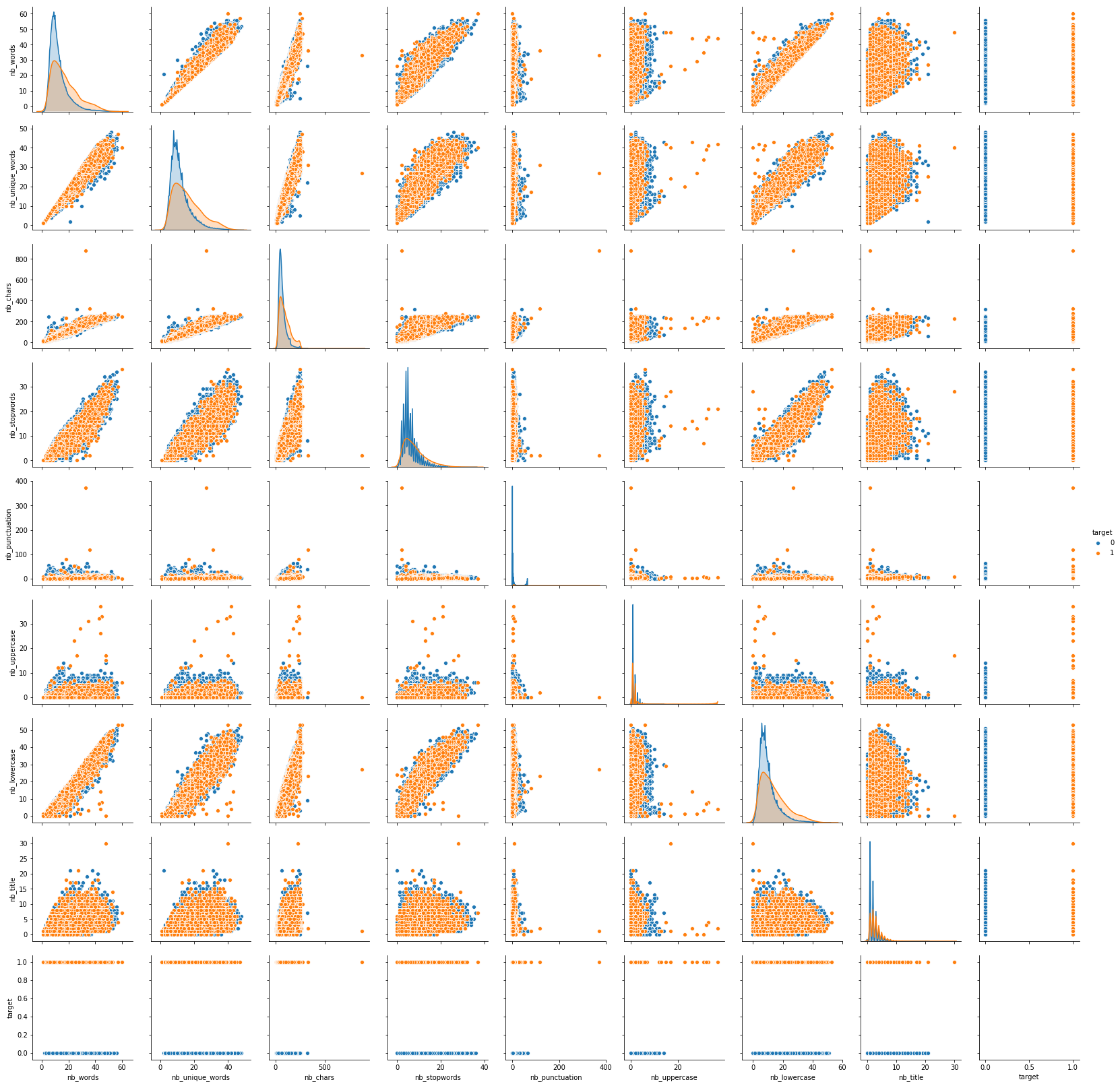
Let’s take a sample - because the data set is quite huge when run locally on a single node - and visualize pair plots :
num_feat = ['nb_words', 'nb_unique_words', 'nb_chars', 'nb_stopwords', \
            'nb_punctuation', 'nb_uppercase', 'nb_lowercase', 'nb_title', 'target']
# side note : remove target if needed later

df_sample = df[num_feat].sample(n=round(df.shape[0]/6), random_state=42)

plt.figure(figsize=(16,10))
sns.pairplot(data=df_sample, hue='target')
plt.show()
<Figure size 1152x720 with 0 Axes>
Basic stats comparison :
df_sample[df_sample['target'] == 0].describe()
| nb_words | nb_unique_words | nb_chars | nb_stopwords | nb_punctuation | nb_uppercase | nb_lowercase | nb_title | target | |
|---|---|---|---|---|---|---|---|---|---|
| count | 204532.000000 | 204532.000000 | 204532.000000 | 204532.000000 | 204532.000000 | 204532.000000 | 204532.000000 | 204532.000000 | 204532.0 |
| mean | 12.509334 | 11.880190 | 68.885475 | 6.043426 | 1.706897 | 0.459860 | 10.035466 | 2.062655 | 0.0 |
| std | 6.751813 | 5.781951 | 36.732624 | 3.620446 | 1.545802 | 0.842419 | 6.172322 | 1.431942 | 0.0 |
| min | 2.000000 | 2.000000 | 10.000000 | 0.000000 | 0.000000 | 0.000000 | 0.000000 | 0.000000 | 0.0 |
| 25% | 8.000000 | 8.000000 | 44.000000 | 4.000000 | 1.000000 | 0.000000 | 6.000000 | 1.000000 | 0.0 |
| 50% | 11.000000 | 10.000000 | 59.000000 | 5.000000 | 1.000000 | 0.000000 | 8.000000 | 2.000000 | 0.0 |
| 75% | 15.000000 | 14.000000 | 83.000000 | 7.000000 | 2.000000 | 1.000000 | 12.000000 | 3.000000 | 0.0 |
| max | 56.000000 | 48.000000 | 319.000000 | 36.000000 | 65.000000 | 14.000000 | 51.000000 | 21.000000 | 0.0 |
df_sample[df_sample['target'] == 1].describe()
| nb_words | nb_unique_words | nb_chars | nb_stopwords | nb_punctuation | nb_uppercase | nb_lowercase | nb_title | target | |
|---|---|---|---|---|---|---|---|---|---|
| count | 13155.000000 | 13155.000000 | 13155.000000 | 13155.000000 | 13155.000000 | 13155.000000 | 13155.000000 | 13155.000000 | 13155.0 |
| mean | 17.338502 | 16.073280 | 98.295325 | 8.063398 | 2.382516 | 0.339187 | 13.960775 | 2.973014 | 1.0 |
| std | 9.697397 | 8.224487 | 55.799960 | 5.056734 | 3.991050 | 1.029390 | 8.770353 | 1.992830 | 0.0 |
| min | 1.000000 | 1.000000 | 7.000000 | 0.000000 | 0.000000 | 0.000000 | 0.000000 | 0.000000 | 1.0 |
| 25% | 10.000000 | 10.000000 | 54.000000 | 4.000000 | 1.000000 | 0.000000 | 7.000000 | 2.000000 | 1.0 |
| 50% | 15.000000 | 14.000000 | 86.000000 | 7.000000 | 2.000000 | 0.000000 | 12.000000 | 3.000000 | 1.0 |
| 75% | 23.000000 | 21.000000 | 130.000000 | 11.000000 | 3.000000 | 0.000000 | 19.000000 | 4.000000 | 1.0 |
| max | 60.000000 | 47.000000 | 878.000000 | 37.000000 | 372.000000 | 37.000000 | 53.000000 | 30.000000 | 1.0 |
Generally speaking, insincere questions are written with more words.
Now with a focus on the distributions, because there is a difference in the spikes between sincere and insincre questions.
plt.figure(figsize=(10,10))
plt.subplot(331)

i=0
for c in num_feat:
    plt.subplot(3, 3, i+1)
    i += 1
    sns.kdeplot(df_sample[df_sample['target'] == 0][c], shade=True)
    sns.kdeplot(df_sample[df_sample['target'] == 1][c], shade=False)
    plt.title(c)

plt.show()
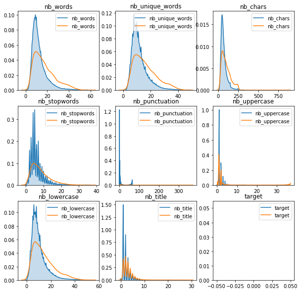
Same conclusion here than shown with stats
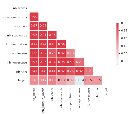
Obviously, many of these indicators are highly correlated each other but not towards the target :
sns.set(style="white")

# Compute the correlation matrix
corr = df_sample[num_feat].corr()

# Generate a mask for the upper triangle
mask = np.zeros_like(corr, dtype=np.bool)
mask[np.triu_indices_from(mask)] = True

# Set up the matplotlib figure
f, ax = plt.subplots(figsize=(7, 6))

# Generate a custom diverging colormap
cmap = sns.diverging_palette(220, 10, as_cmap=True)

# Draw the heatmap with the mask and correct aspect ratio
sns.heatmap(corr, mask=mask, cmap=cmap, vmax=.3, center=0,
            square=True, linewidths=.5, annot=True, cbar_kws={"shrink": .5})
<matplotlib.axes._subplots.AxesSubplot at 0x7f0d99b5eba8>
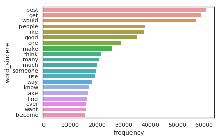
What are the most frequent words for each type of question ?
class Vocabulary(object):
    # credits : Shankar G see https://www.kaggle.com/kaosmonkey/visualize-sincere-vs-insincere-words

    def __init__(self):
        self.vocab = {}
        self.STOPWORDS = set()
        self.STOPWORDS = set(stopwords.words('english'))

    def build_vocab(self, lines):
        for line in lines:
            for word in line.split(' '):
                word = word.lower()
                if (word in self.STOPWORDS):
                    continue
                if (word not in self.vocab):
                    self.vocab[word] = 0
                self.vocab[word] +=1

    def generate_ngrams(text, n_gram=1):
        """arg: text, n_gram"""
        token = [token for token in text.lower().split(" ") if token != "" if token not in STOPWORDS]
        ngrams = zip(*[token[i:] for i in range(n_gram)])
        return [" ".join(ngram) for ngram in ngrams]

    def horizontal_bar_chart(df, color):
        trace = go.Bar(
            y=df["word"].values[::-1],
            x=df["wordcount"].values[::-1],
            showlegend=False,
            orientation = 'h',
            marker=dict(
            color=color,
            ),
        )
        return trace
sincere_vocab = Vocabulary()
sincere_vocab.build_vocab(df[df['target'] == 0]['question_text'])
sincere_vocabulary = sorted(sincere_vocab.vocab.items(), reverse=True, key=lambda kv: kv[1])

df_sincere_vocab = pd.DataFrame(sincere_vocabulary, columns=['word_sincere', 'frequency'])
sns.barplot(y='word_sincere', x='frequency', data=df_sincere_vocab[:20])
<matplotlib.axes._subplots.AxesSubplot at 0x7f0d99d79ac8>
insincere_vocab = Vocabulary()
insincere_vocab.build_vocab(df[df['target'] == 1]['question_text'])
insincere_vocabulary = sorted(insincere_vocab.vocab.items(), reverse=True, key=lambda kv: kv[1])

df_insincere_vocab = pd.DataFrame(insincere_vocabulary, columns=['word_insincere', 'frequency'])
sns.barplot(y='word_insincere', x='frequency', data=df_insincere_vocab[:20])
<matplotlib.axes._subplots.AxesSubplot at 0x7f0d86abfa58>
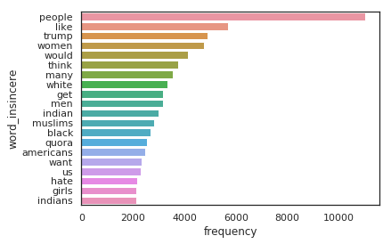
As we can clearly see there are certain words (swear words, discriminatory words based on race, political figures etc) that show up a lot in insincere sentences.
Text processing & model training
Metric : F-score
The most appropriated metric is F1-score. Explanation from Wikipedia:
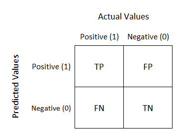
“In statistical analysis of binary classification, the F1 score (also F-score or F-measure) is a measure of a test’s accuracy. It considers both the precision p and the recall r of the test to compute the score: p is the number of correct positive results divided by the number of all positive results returned by the classifier, and r is the number of correct positive results divided by the number of all relevant samples (all samples that should have been identified as positive). The F1 score is the harmonic mean of the precision and recall, where an F1 score reaches its best value at 1 (perfect precision and recall) and worst at 0.”
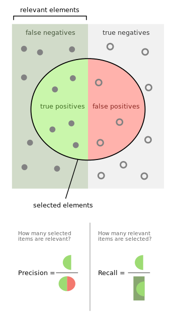
we’ll also use a confusion matrix the most import part is the recall for insincere questions (class 1), because if the recall isn’t good enough, the f1-score won’t satisfying either. Here are mathematical definitions :


def get_fscore_matrix(fitted_clf, model_name):
    print(model_name, ' :')

    # get classes predictions for the classification report
    y_train_pred, y_pred = fitted_clf.predict(X_train), fitted_clf.predict(X_test)
    print(classification_report(y_test, y_pred), '\n') # target_names=y

    # computes probabilities keep the ones for the positive outcome only
    print(f'F1-score = {f1_score(y_test, y_pred):.2f}')
Text processing
# if needed the first time
# import nltk
# nltk.download('punkt')
Process : - tokenization - keeping only alphanumeriacl characters - removing stop words (punctuation etc…) - stemming or lemmatization.
Tokenization : Given a character sequence and a defined document unit, tokenization is the task of chopping it up into pieces, called tokens , perhaps at the same time throwing away certain characters, such as punctuation
Stemming vs. lemmatization : The aim of both processes is the same: reducing the inflectional forms of each word into a common base or root.
Stemming algorithms work by cutting off the end or the beginning of the word, taking into account a list of common prefixes and suffixes that can be found in an inflected word. This indiscriminate cutting can be successful in some occasions, but not always, and that is why we affirm that this approach presents some limitations.
Lemmatization, on the other hand, takes into consideration the morphological analysis of the words. To do so, it is necessary to have detailed dictionaries which the algorithm can look through to link the form back to its lemma.
df = df[['question_text', 'target']]

def text_processing(local_df):
    """ return the dataframe with tokens stemmetized without numerical values & stopwords """
    stemmer = PorterStemmer()
    # Perform preprocessing
    local_df['txt_processed'] = local_df['question_text'].apply(lambda df: word_tokenize(df))
    local_df['txt_processed'] = local_df['txt_processed'].apply(lambda x: [item for item in x if item.isalpha()])
    local_df['txt_processed'] = local_df['txt_processed'].apply(lambda x: [item for item in x if item not in stop_words])
    local_df['txt_processed'] = local_df['txt_processed'].apply(lambda x: [stemmer.stem(item) for item in x])
    return local_df
df = text_processing(df)
df.tail(2)
| question_text | target | txt_processed | |
|---|---|---|---|
| 1306120 | How can one start a research project based on ... | 0 | [how, one, start, research, project, base, bio... |
| 1306121 | Who wins in a battle between a Wolverine and a... | 0 | [who, win, battl, wolverin, puma] |
First method : text similarity using TF-IDF
vectorizer = TfidfVectorizer(lowercase=False, analyzer=lambda x: x, min_df=0.01, max_df=0.999)
# min_df & max_df param added for less memory usage

tf_idf = vectorizer.fit_transform(df['txt_processed']).toarray()
pd.DataFrame(tf_idf, columns=vectorizer.get_feature_names()).head()
| Do | I | If | Is | are | becom | best | better | book | can | ... | where | whi | which | who | will | without | work | world | would | year | |
|---|---|---|---|---|---|---|---|---|---|---|---|---|---|---|---|---|---|---|---|---|---|
| 0 | 0.000000 | 0.000000 | 0.0 | 0.0 | 0.0 | 0.0 | 0.0 | 0.0 | 0.0 | 0.00000 | ... | 0.0 | 0.000000 | 0.0 | 0.0 | 0.0 | 0.0 | 0.0 | 0.0 | 0.000000 | 0.0 |
| 1 | 0.606073 | 0.000000 | 0.0 | 0.0 | 0.0 | 0.0 | 0.0 | 0.0 | 0.0 | 0.00000 | ... | 0.0 | 0.000000 | 0.0 | 0.0 | 0.0 | 0.0 | 0.0 | 0.0 | 0.554503 | 0.0 |
| 2 | 0.000000 | 0.000000 | 0.0 | 0.0 | 0.0 | 0.0 | 0.0 | 0.0 | 0.0 | 0.00000 | ... | 0.0 | 0.416315 | 0.0 | 0.0 | 0.0 | 0.0 | 0.0 | 0.0 | 0.000000 | 0.0 |
| 3 | 0.000000 | 0.000000 | 0.0 | 0.0 | 0.0 | 0.0 | 0.0 | 0.0 | 0.0 | 0.00000 | ... | 0.0 | 0.000000 | 0.0 | 0.0 | 0.0 | 0.0 | 0.0 | 0.0 | 0.000000 | 0.0 |
| 4 | 0.000000 | 0.360439 | 0.0 | 0.0 | 0.0 | 0.0 | 0.0 | 0.0 | 0.0 | 0.56217 | ... | 0.0 | 0.000000 | 0.0 | 0.0 | 0.0 | 0.0 | 0.0 | 0.0 | 0.000000 | 0.0 |
5 rows × 76 columns
# Split the data
X_train, X_test, y_train, y_test = train_test_split(tf_idf, df['target'], test_size=0.2, random_state=42)
XGBoost Classifier without weigths
model = XGBClassifier(objective="binary:logistic")
model.fit(X_train, y_train)
get_fscore_matrix(model, 'XGB Clf withOUT weights')
XGB Clf withOUT weights  :
              precision    recall  f1-score   support

           0       0.94      1.00      0.97    245369
           1       0.61      0.05      0.10     15856

   micro avg       0.94      0.94      0.94    261225
   macro avg       0.78      0.53      0.53    261225
weighted avg       0.92      0.94      0.92    261225


F1-score = 0.10
XGBoost Classifier with weigths
ratio = ((len(y_train) - y_train.sum()) - y_train.sum()) / y_train.sum()
ratio
14.086722911598978
model = XGBClassifier(objective="binary:logistic", scale_pos_weight=ratio)
model.fit(X_train, y_train)
get_fscore_matrix(model, 'XGB Clf WITH weights')
XGB Clf WITH weights  :
              precision    recall  f1-score   support

           0       0.98      0.81      0.89    245369
           1       0.19      0.68      0.30     15856

   micro avg       0.81      0.81      0.81    261225
   macro avg       0.58      0.75      0.59    261225
weighted avg       0.93      0.81      0.85    261225


F1-score = 0.30
Now LGBM with weights
model = lgb.LGBMClassifier(n_jobs = -1, class_weight={0:y_train.sum(), 1:len(y_train) - y_train.sum()})
model.fit(X_train, y_train)
get_fscore_matrix(model, 'LGBM weighted')
LGBM weighted  :
              precision    recall  f1-score   support

           0       0.98      0.73      0.84    245369
           1       0.16      0.80      0.26     15856

   micro avg       0.73      0.73      0.73    261225
   macro avg       0.57      0.76      0.55    261225
weighted avg       0.93      0.73      0.80    261225


F1-score = 0.26
LogisticRegression
model = LogisticRegression(class_weight={0:y_train.sum(), 1:len(y_train) - y_train.sum()}, C=0.5, max_iter=100, n_jobs=-1)
model.fit(X_train, y_train)
get_fscore_matrix(model, 'LogisticRegression')
LogisticRegression  :
              precision    recall  f1-score   support

           0       0.98      0.72      0.83    245369
           1       0.15      0.79      0.26     15856

   micro avg       0.73      0.73      0.73    261225
   macro avg       0.57      0.75      0.54    261225
weighted avg       0.93      0.73      0.80    261225


F1-score = 0.26
Second approach : a CountVectorizer / Logistic Regression pipeline
Convert a collection of text documents to a matrix of token counts
This implementation produces a sparse representation of the counts using scipy.sparse.csr_matrix.
df['str_processed'] = df['txt_processed'].apply(lambda x: " ".join(x))
df.head(2)
| question_text | target | txt_processed | str_processed | |
|---|---|---|---|---|
| 0 | How did Quebec nationalists see their province... | 0 | [how, quebec, nationalist, see, provinc, nation] | how quebec nationalist see provinc nation |
| 1 | Do you have an adopted dog, how would you enco... | 0 | [Do, adopt, dog, would, encourag, peopl, adopt... | Do adopt dog would encourag peopl adopt shop |
pipeline = Pipeline([("cv", CountVectorizer(analyzer="word", ngram_range=(1,4), max_df=0.9)),
                     ("clf", LogisticRegression(solver="saga", class_weight="balanced", C=0.45, max_iter=250, verbose=1, n_jobs=-1))])
X_train, X_test, y_train, y_test = train_test_split(df['str_processed'], df.target, test_size=0.2, stratify = df.target.values)
lr_model = pipeline.fit(X_train, y_train)
lr_model
[Parallel(n_jobs=-1)]: Using backend ThreadingBackend with 8 concurrent workers.


max_iter reached after 431 seconds


/home/sunflowa/Anaconda/lib/python3.7/site-packages/sklearn/linear_model/sag.py:334: ConvergenceWarning: The max_iter was reached which means the coef_ did not converge
  "the coef_ did not converge", ConvergenceWarning)
[Parallel(n_jobs=-1)]: Done   1 out of   1 | elapsed:  7.3min finished


Pipeline(memory=None,
     steps=[('cv', CountVectorizer(analyzer='word', binary=False, decode_error='strict',
        dtype=<class 'numpy.int64'>, encoding='utf-8', input='content',
        lowercase=True, max_df=0.9, max_features=None, min_df=1,
        ngram_range=(1, 4), preprocessor=None, stop_words=None,
        strip_a...penalty='l2', random_state=None,
          solver='saga', tol=0.0001, verbose=1, warm_start=False))])
get_fscore_matrix(lr_model, 'lr_pipe')
lr_pipe  :
              precision    recall  f1-score   support

           0       1.00      0.98      0.99    245063
           1       0.75      0.94      0.83     16162

   micro avg       0.98      0.98      0.98    261225
   macro avg       0.87      0.96      0.91    261225
weighted avg       0.98      0.98      0.98    261225


F1-score = 0.83
Conclusion, submission and opening
- First we have used TF-IDF, but the least we can say : this is not really efficient, the recall for insincere question isn’t good at all, so this seems to not be the right way to go…
- Instead, using CountVectorizer with a Logistic Regression is more efficient.
Now let’s see what will be the submission score ?
pd.read_csv("../input/quora-insincere-questions-classification/sample_submission.csv").head(2)
| qid | prediction | |
|---|---|---|
| 0 | 0000163e3ea7c7a74cd7 | 0 |
| 1 | 00002bd4fb5d505b9161 | 0 |
df_test = pd.read_csv("../input/quora-insincere-questions-classification/test.csv", index_col='qid')
df_test.tail(2)
| question_text | |
|---|---|
| qid | |
| ffffb1f7f1a008620287 | What are the causes of refraction of light? |
| fffff85473f4699474b0 | Climate change is a worrying topic. How much t... |
df_test = text_processing(df_test)
df_test['str_processed'] = df_test['txt_processed'].apply(lambda x: " ".join(x))
df_test.head(2)
| question_text | txt_processed | str_processed | |
|---|---|---|---|
| qid | |||
| 0000163e3ea7c7a74cd7 | Why do so many women become so rude and arroga... | [whi, mani, women, becom, rude, arrog, get, li... | whi mani women becom rude arrog get littl bit ... |
| 00002bd4fb5d505b9161 | When should I apply for RV college of engineer... | [when, I, appli, RV, colleg, engin, bm, colleg... | when I appli RV colleg engin bm colleg engin s... |
y_pred_final = lr_model.predict(df_test['str_processed'])
y_pred_final
array([1, 0, 0, ..., 0, 0, 0])
df_submission = pd.DataFrame({"qid":df_test.index, "prediction":y_pred_final})
df_submission.head()
| qid | prediction | |
|---|---|---|
| 0 | 0000163e3ea7c7a74cd7 | 1 |
| 1 | 00002bd4fb5d505b9161 | 0 |
| 2 | 00007756b4a147d2b0b3 | 0 |
| 3 | 000086e4b7e1c7146103 | 0 |
| 4 | 0000c4c3fbe8785a3090 | 0 |
df_submission.to_csv('submission.csv', index=False)
Submission score = 0.61580 not that bad !
CREDITS : all the people mentionned above and especially amokrane & moneynass for their inspiring work ! thanks :)
-> IN THE 2nd PART I’LL USE WORD ENBEDDINGS !
