

How to Forecast Real Estate Prices?
California Housing Prices
Prediction of Median house prices for California districts derived from the 1990 census.
Header by Vita Vilcina
Context
This is the dataset used in the second chapter of Aurélien Géron’s recent book ‘Hands-On Machine learning with Scikit-Learn and TensorFlow’. It serves as an excellent introduction to implementing machine learning algorithms because it requires rudimentary data cleaning, has an easily understandable list of variables and sits at an optimal size between being to toyish and too cumbersome.
The data contains information from the 1990 California census. So although it may not help you with predicting current housing prices like the Zillow Zestimate dataset, it does provide an accessible introductory dataset for teaching people about the basics of machine learning.
Acknowledgements
Please refer to the Kaggle challenge web page
Inspiration
predict a real estate price
Exploratory Data Analysis
import pandas as pd
import numpy as np
import matplotlib.pyplot as plt
import seaborn as sns
import os
import folium
from sklearn.model_selection import train_test_split
from sklearn.metrics import mean_squared_error
from sklearn.linear_model import Lasso, LinearRegression, Ridge, RANSACRegressor, SGDRegressor
from sklearn.ensemble import AdaBoostRegressor
from sklearn.svm import SVR
file_path = os.path.join('input', 'house_big.csv')
df = pd.read_csv(file_path)
df.head()
| longitude | latitude | housing_median_age | total_rooms | total_bedrooms | population | households | median_income | median_house_value | ocean_proximity | |
|---|---|---|---|---|---|---|---|---|---|---|
| 0 | -122.23 | 37.88 | 41.0 | 880.0 | 129.0 | 322.0 | 126.0 | 8.3252 | 452600.0 | NEAR BAY |
| 1 | -122.22 | 37.86 | 21.0 | 7099.0 | 1106.0 | 2401.0 | 1138.0 | 8.3014 | 358500.0 | NEAR BAY |
| 2 | -122.24 | 37.85 | 52.0 | 1467.0 | 190.0 | 496.0 | 177.0 | 7.2574 | 352100.0 | NEAR BAY |
| 3 | -122.25 | 37.85 | 52.0 | 1274.0 | 235.0 | 558.0 | 219.0 | 5.6431 | 341300.0 | NEAR BAY |
| 4 | -122.25 | 37.85 | 52.0 | 1627.0 | 280.0 | 565.0 | 259.0 | 3.8462 | 342200.0 | NEAR BAY |
df.shape
(20640, 10)
Content
The data pertains to the houses found in a given California district and some summary stats about them based on the 1990 census data. Be warned the data aren’t cleaned so there are some preprocessing steps required! The columns are as follows, their names are pretty self explanitory:
- longitude
- latitude
- housing_median_age
- total_rooms
- total_bedrooms
- population
- households
- median_income
- median_house_value
- ocean_proximity
df.info()
<class 'pandas.core.frame.DataFrame'>
RangeIndex: 20640 entries, 0 to 20639
Data columns (total 10 columns):
longitude 20640 non-null float64
latitude 20640 non-null float64
housing_median_age 20640 non-null float64
total_rooms 20640 non-null float64
total_bedrooms 20433 non-null float64
population 20640 non-null float64
households 20640 non-null float64
median_income 20640 non-null float64
median_house_value 20640 non-null float64
ocean_proximity 20640 non-null object
dtypes: float64(9), object(1)
memory usage: 1.6+ MB
There are few missing value int the ‘total_bedrooms’ column. Now let’s see the basic stats for the numerical columns:
df.describe()
| longitude | latitude | housing_median_age | total_rooms | total_bedrooms | population | households | median_income | median_house_value | |
|---|---|---|---|---|---|---|---|---|---|
| count | 20640.000000 | 20640.000000 | 20640.000000 | 20640.000000 | 20433.000000 | 20640.000000 | 20640.000000 | 20640.000000 | 20640.000000 |
| mean | -119.569704 | 35.631861 | 28.639486 | 2635.763081 | 537.870553 | 1425.476744 | 499.539680 | 3.870671 | 206855.816909 |
| std | 2.003532 | 2.135952 | 12.585558 | 2181.615252 | 421.385070 | 1132.462122 | 382.329753 | 1.899822 | 115395.615874 |
| min | -124.350000 | 32.540000 | 1.000000 | 2.000000 | 1.000000 | 3.000000 | 1.000000 | 0.499900 | 14999.000000 |
| 25% | -121.800000 | 33.930000 | 18.000000 | 1447.750000 | 296.000000 | 787.000000 | 280.000000 | 2.563400 | 119600.000000 |
| 50% | -118.490000 | 34.260000 | 29.000000 | 2127.000000 | 435.000000 | 1166.000000 | 409.000000 | 3.534800 | 179700.000000 |
| 75% | -118.010000 | 37.710000 | 37.000000 | 3148.000000 | 647.000000 | 1725.000000 | 605.000000 | 4.743250 | 264725.000000 |
| max | -114.310000 | 41.950000 | 52.000000 | 39320.000000 | 6445.000000 | 35682.000000 | 6082.000000 | 15.000100 | 500001.000000 |
df.ocean_proximity.value_counts()
<1H OCEAN 9136
INLAND 6551
NEAR OCEAN 2658
NEAR BAY 2290
ISLAND 5
Name: ocean_proximity, dtype: int64
Cleaning data
df.duplicated().sum()
0
df.isnull().sum()
longitude 0
latitude 0
housing_median_age 0
total_rooms 0
total_bedrooms 207
population 0
households 0
median_income 0
median_house_value 0
ocean_proximity 0
dtype: int64
print(f'percentage of missing values: {df.total_bedrooms.isnull().sum() / df.shape[0] * 100 :.2f}%')
percentage of missing values: 1.00%
df = df.fillna(df.median())
df.isnull().sum()
longitude 0
latitude 0
housing_median_age 0
total_rooms 0
total_bedrooms 0
population 0
households 0
median_income 0
median_house_value 0
ocean_proximity 0
dtype: int64
Dealing with geospatial infos
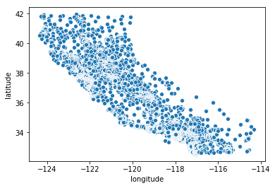
Visualization of the data in a scatter plot in a “geographic way”
sns.scatterplot(df.longitude, df.latitude)
<matplotlib.axes._subplots.AxesSubplot at 0x7f244cbecb00>
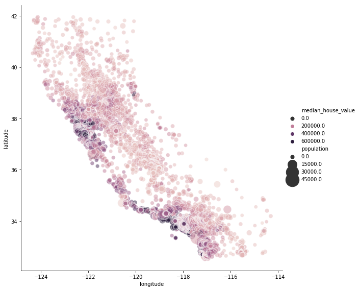
Same plot but this time with a varying size of the data points based on population variable and a different color depending of the real estate price (median_house_value)
sns.relplot(x="longitude", y="latitude", hue="median_house_value", size="population", alpha=.5,\
sizes=(50, 700), data=df, height=8)
plt.show()
# Create a map with folium centered at the mean latitude and longitude
cali_map = folium.Map(location=[35.6, -117], zoom_start=6)
# Display the map
display(cali_map)
# Add markers for each rows
for i in range(df.shape[0]):
folium.Marker((float(df.iloc[i, 1]), float(df.iloc[i, 0]))).add_to(cali_map)
# Display the map
display(cali_map)
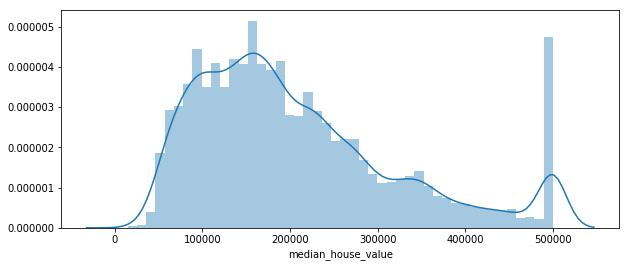
Target analysis
plt.figure(figsize=(10, 4))
sns.distplot(df.median_house_value)
plt.show()
/home/sunflowa/anaconda3/lib/python3.7/site-packages/scipy/stats/stats.py:1713: FutureWarning: Using a non-tuple sequence for multidimensional indexing is deprecated; use `arr[tuple(seq)]` instead of `arr[seq]`. In the future this will be interpreted as an array index, `arr[np.array(seq)]`, which will result either in an error or a different result.
return np.add.reduce(sorted[indexer] * weights, axis=axis) / sumval
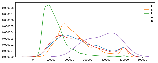
Variations depending on the proximity with ocean
df.ocean_proximity.unique()
array(['NEAR BAY', '<1H OCEAN', 'INLAND', 'NEAR OCEAN', 'ISLAND'],
dtype=object)
plt.figure(figsize=(10, 4))
for prox in df.ocean_proximity.unique():
sns.kdeplot(data=df[df.ocean_proximity == prox].median_house_value)
plt.legend(prox)
plt.show()
Other analysis
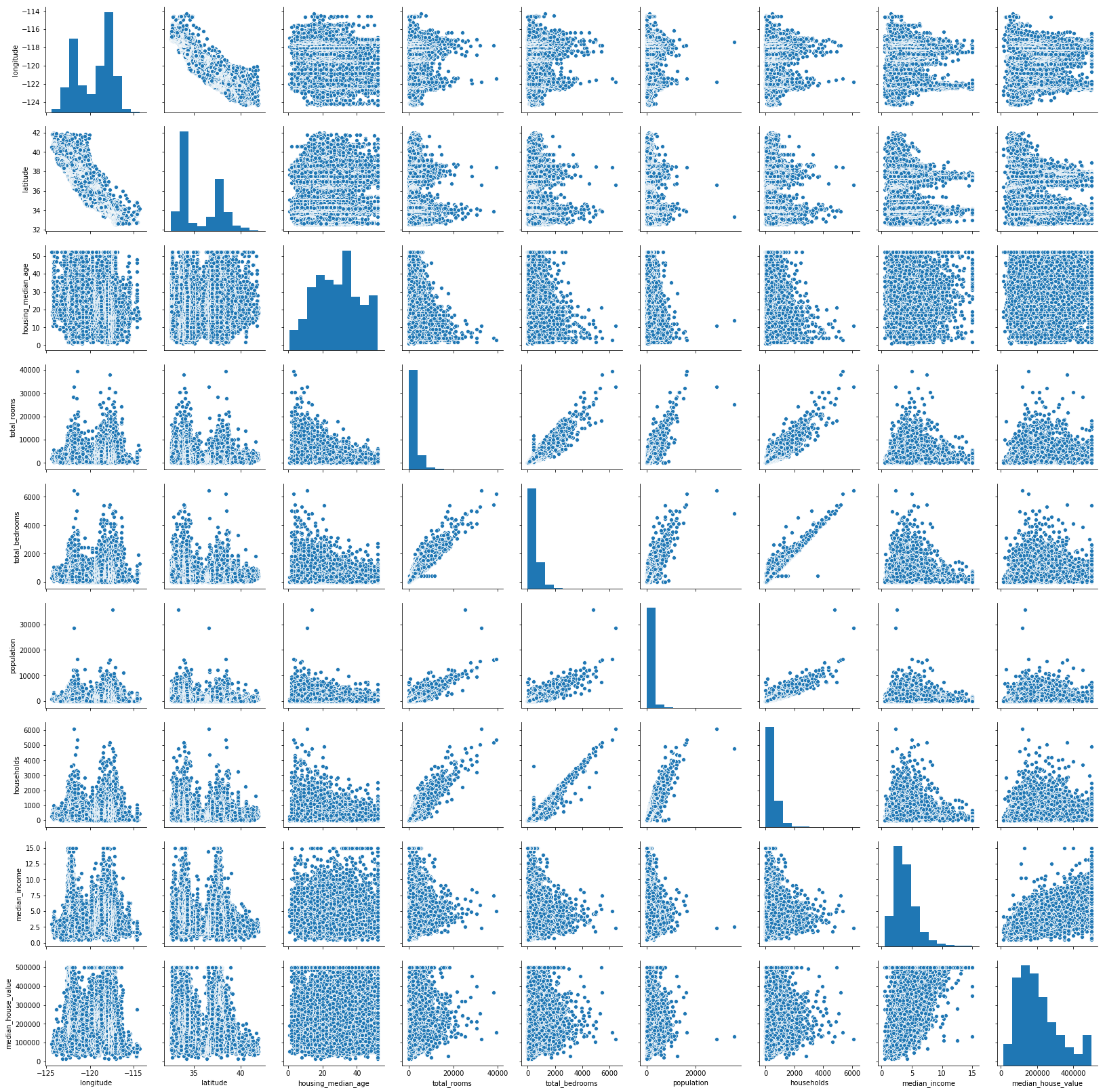
sns.pairplot(df)
plt.show()
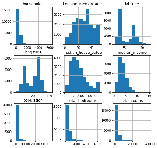
df.hist(figsize=(8, 8))
plt.show()
Correlations
corr = df.corr()
corr
| longitude | latitude | housing_median_age | total_rooms | total_bedrooms | population | households | median_income | median_house_value | |
|---|---|---|---|---|---|---|---|---|---|
| longitude | 1.000000 | -0.924664 | -0.108197 | 0.044568 | 0.069120 | 0.099773 | 0.055310 | -0.015176 | -0.045967 |
| latitude | -0.924664 | 1.000000 | 0.011173 | -0.036100 | -0.066484 | -0.108785 | -0.071035 | -0.079809 | -0.144160 |
| housing_median_age | -0.108197 | 0.011173 | 1.000000 | -0.361262 | -0.319026 | -0.296244 | -0.302916 | -0.119034 | 0.105623 |
| total_rooms | 0.044568 | -0.036100 | -0.361262 | 1.000000 | 0.927058 | 0.857126 | 0.918484 | 0.198050 | 0.134153 |
| total_bedrooms | 0.069120 | -0.066484 | -0.319026 | 0.927058 | 1.000000 | 0.873535 | 0.974366 | -0.007617 | 0.049457 |
| population | 0.099773 | -0.108785 | -0.296244 | 0.857126 | 0.873535 | 1.000000 | 0.907222 | 0.004834 | -0.024650 |
| households | 0.055310 | -0.071035 | -0.302916 | 0.918484 | 0.974366 | 0.907222 | 1.000000 | 0.013033 | 0.065843 |
| median_income | -0.015176 | -0.079809 | -0.119034 | 0.198050 | -0.007617 | 0.004834 | 0.013033 | 1.000000 | 0.688075 |
| median_house_value | -0.045967 | -0.144160 | 0.105623 | 0.134153 | 0.049457 | -0.024650 | 0.065843 | 0.688075 | 1.000000 |
# Generate a mask for the upper triangle
mask = np.zeros_like(corr, dtype=np.bool)
mask[np.triu_indices_from(mask)] = True
# Set up the matplotlib figure
f, ax = plt.subplots(figsize=(8, 6))
# Generate a custom diverging colormap
cmap = sns.diverging_palette(220, 10, as_cmap=True)
# Draw the heatmap with the mask and correct aspect ratio
sns.heatmap(corr, mask=mask, cmap=cmap, vmax=.3, center=0,
square=True, linewidths=.5, cbar_kws={"shrink": .5}, annot=True)
<matplotlib.axes._subplots.AxesSubplot at 0x7f243ec37898>
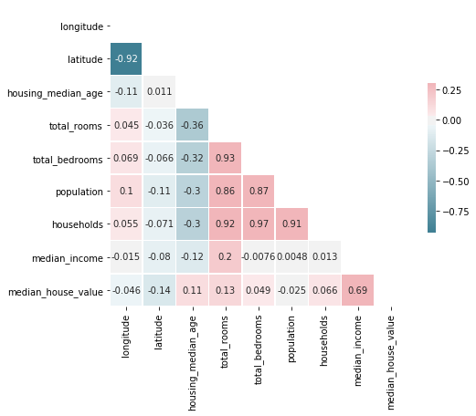
- lat and log are highly positively correlated
- total_bedrooms, population and householdsare highly positively correlated too
- median_income and median_house_value are also positively correlated
which make sense.
Models training and predictions
Data preparation
Label encoding of categorical feature (ocean proximity)
df = pd.get_dummies(data=df, columns=['ocean_proximity'], drop_first=False)
df.head()
| longitude | latitude | housing_median_age | total_rooms | total_bedrooms | population | households | median_income | median_house_value | ocean_proximity_<1H OCEAN | ocean_proximity_INLAND | ocean_proximity_ISLAND | ocean_proximity_NEAR BAY | ocean_proximity_NEAR OCEAN | |
|---|---|---|---|---|---|---|---|---|---|---|---|---|---|---|
| 0 | -122.23 | 37.88 | 41.0 | 880.0 | 129.0 | 322.0 | 126.0 | 8.3252 | 452600.0 | 0 | 0 | 0 | 1 | 0 |
| 1 | -122.22 | 37.86 | 21.0 | 7099.0 | 1106.0 | 2401.0 | 1138.0 | 8.3014 | 358500.0 | 0 | 0 | 0 | 1 | 0 |
| 2 | -122.24 | 37.85 | 52.0 | 1467.0 | 190.0 | 496.0 | 177.0 | 7.2574 | 352100.0 | 0 | 0 | 0 | 1 | 0 |
| 3 | -122.25 | 37.85 | 52.0 | 1274.0 | 235.0 | 558.0 | 219.0 | 5.6431 | 341300.0 | 0 | 0 | 0 | 1 | 0 |
| 4 | -122.25 | 37.85 | 52.0 | 1627.0 | 280.0 | 565.0 | 259.0 | 3.8462 | 342200.0 | 0 | 0 | 0 | 1 | 0 |
feat_removed = ['median_house_value']
# removed
#['longitude', 'latitude', 'housing_median_age', 'total_rooms', 'total_bedrooms', 'population', 'households', 'median_income',
#'median_house_value', 'ocean_proximity']
y = df.median_house_value
X = df.drop(columns=feat_removed)
X.shape, y.shape
((20640, 13), (20640,))
X_train, X_test, y_train, y_test = train_test_split(X, y, test_size=0.2)
Metric RMSE root mean squared error
Root Mean Square Error (RMSE) is the standard deviation of the residuals (prediction errors). Residuals are a measure of how far from the regression line data points are; RMSE is a measure of how spread out these residuals are. In other words, it tells you how concentrated the data is around the line of best fit. Root mean square error is commonly used in climatology, forecasting, and regression analysis to verify experimental results.

def calculate_rmse(model, model_name):
model.fit(X_train, y_train)
y_pred, y_pred_train = model.predict(X_test), model.predict(X_train)
rmse_test, rmse_train = np.sqrt(mean_squared_error(y_test, y_pred)), np.sqrt(mean_squared_error(y_train, y_pred_train))
print(model_name, f' RMSE on train: {rmse_train:.0f}, on test: {rmse_test:.0f}')
return rmse_test
Linear Regression
lr = LinearRegression()
lr_err = calculate_rmse(lr, 'Linear Reg')
Linear Reg RMSE on train: 68533, on test: 69932
RANSAC Regressor
ra = RANSACRegressor()
ra_err = calculate_rmse(ra, 'RANSAC Reg')
RANSAC Reg RMSE on train: 78281, on test: 78795
Lasso
la = Lasso()
la_err = calculate_rmse(la, 'Lasso Reg')
Lasso Reg RMSE on train: 68533, on test: 69932
/home/sunflowa/anaconda3/lib/python3.7/site-packages/sklearn/linear_model/coordinate_descent.py:492: ConvergenceWarning: Objective did not converge. You might want to increase the number of iterations. Fitting data with very small alpha may cause precision problems.
ConvergenceWarning)
SGD Regressor
sg = SGDRegressor()
sg_err = calculate_rmse(sg, 'SGD Reg')
SGD Reg RMSE on train: 2939589866401599, on test: 2954302199978100
/home/sunflowa/anaconda3/lib/python3.7/site-packages/sklearn/linear_model/stochastic_gradient.py:166: FutureWarning: max_iter and tol parameters have been added in SGDRegressor in 0.19. If both are left unset, they default to max_iter=5 and tol=None. If tol is not None, max_iter defaults to max_iter=1000. From 0.21, default max_iter will be 1000, and default tol will be 1e-3.
FutureWarning)
Ridge
ri = SGDRegressor()
ri_err = calculate_rmse(ri, 'Ridge')
Ridge RMSE on train: 24125952802617160, on test: 24256192059939448
/home/sunflowa/anaconda3/lib/python3.7/site-packages/sklearn/linear_model/stochastic_gradient.py:166: FutureWarning: max_iter and tol parameters have been added in SGDRegressor in 0.19. If both are left unset, they default to max_iter=5 and tol=None. If tol is not None, max_iter defaults to max_iter=1000. From 0.21, default max_iter will be 1000, and default tol will be 1e-3.
FutureWarning)
AdaBoostRegressor
ad = AdaBoostRegressor()
ad_err = calculate_rmse(ad, 'AdaBoostRegressor')
AdaBoostRegressor RMSE on train: 86734, on test: 86345
SVR
sv = SVR()
sv_err = calculate_rmse(sv, 'SVR')
/home/sunflowa/anaconda3/lib/python3.7/site-packages/sklearn/svm/base.py:196: FutureWarning: The default value of gamma will change from 'auto' to 'scale' in version 0.22 to account better for unscaled features. Set gamma explicitly to 'auto' or 'scale' to avoid this warning.
"avoid this warning.", FutureWarning)
SVR RMSE on train: 118660, on test: 117282
Results comparison
df_score = pd.DataFrame({'Model':['Linear Reg', 'RANSAC Reg', 'Lasso Reg', 'AdaBoost', 'SVR'],
'RMSE':[lr_err, ra_err, la_err, ad_err, sv_err]})
ax = df_score.plot.barh(y='RMSE', x='Model')
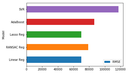
Lasso and the Linear Reg are the winners ! Surprisingly the RSME is a little lower for the best models when we keep features such as lat/long and ‘total_bedrooms’, ‘population’.